LEVEL-0: APPRENTICE
Basics of C++
Introduction to C++

INTRODUCTION TO PROGRAMMING LANGUAGES:
A program is a set of instructions that tells a computer what to do in order to come up with a solution to a particular problem. Programs are written using a programming language.A programming language is a formal language designed to communicate instructions to a computer. There are two major types of programming languages: low-level languages and high-level languages.
TYPES OF LANGUAGES:
Low-Level Languages : Low-level languages are referred to as 'low' because they are very close to how different hardware elements of a computer actually communicate with each other. Low-level languages are machine oriented and require extensive knowledge of computer hardware and its configuration. There are two categories of low-level languages: machine language and assembly language.
Machine language : or machine code, is the only language that is directly understood by the computer, and it does not need to be translated. All instructions use binary notation and are written as a string of 1s and 0s. A program instruction in machine language may look something like this:

However, binary notation is very difficult for humans to understand. This is where assembly languages come in.
An assembly language : is the first step to improve programming structure and make machine language more readable by humans. An assembly language consists of a set of symbols and letters. A translator is required to translate the assembly language to machine language called the 'assembler.' While easier than machine code, assembly languages are still pretty difficult to understand. This is why high-level languages have been developed.
High-Level Languages : A high-level language is a programming language that uses English and mathematical symbols, like +, -, % and many others, in its instructions. When using the term 'programming languages,' most people are actually referring to high-level languages. High-level languages are the languages most often used by programmers to write programs. Examples of high-level languages are C++, Fortran, Java and Python. Learning a high-level language is not unlike learning another human language - you need to learn vocabulary and grammar so you can make sentences. To learn a programming language, you need to learn commands, syntax and logic, which correspond closely to vocabulary and grammar. The code of most high-level languages is portable and the same code can run on different hardware without modification. Both machine code and assembly languages are hardware specific which means that the machine code used to run a program on one specific computer needs to be modified to run on another computer. A high-level language cannot be understood directly by a computer, and it needs to be translated into machine code. There are two ways to do this, and they are related to how the program is executed: a high-level language can be compiled or interpreted.
COMPILER VS INTERPRETER
A compiler is a computer program that translates a program written in a high-level language to the machine language of a computer.
The high-level program is referred to as 'the source code.' The compiler is used to translate source code into machine code or compiled code. This does not yet use any of the input data. When the compiled code is executed, referred to as 'running the program,' the program processes the input data to produce the desired output.
An interpreter is a computer program that directly executes instructions written in a programming language, without requiring them previously to have been compiled into a machine language program.
HOW TO START WRITING PROGRAMS?
Algorithm:
Algorithm is a step-by-step procedure, which defines a set of instructions to be executed in a certain order to get the desired output. Algorithms are generally created independent of underlying languages, i.e. an algorithm can be implemented in more than one programming language.
Qualities of a good algorithm
1. Input and output should be defined precisely.
2. Each step in the algorithm should be clear and unambiguous.
3. An algorithm shouldn’t include computer codes. Instead it should be written in such a way that it can be used in different programming languages. Good, logical programming is developed through good pre-code planning and organization. This is assisted by the use of pseudocode and program flowcharts.
Flowcharts:
Flowcharts are written with program flow from the top of a page to the bottom. Each command is placed in a box of the appropriate shape, and arrows are used to direct program flow.
1.The first figure is oval. Also could be met as an “ellipse”, ”circle”, but it has the same meaning. This is the first and the last symbol in every flow chart. I like to use ellipses for “begin” and “end”. When I divide an algorithm in several parts I use small circles for the start/end of each part.
2.You will use a rectangle to perform an action (also called "statement"). More precisely, we use them for assignment statements - when you change a value of a variable.
3.The parallelogram flowchart symbol serves for input/output(I/O) to/from the program.
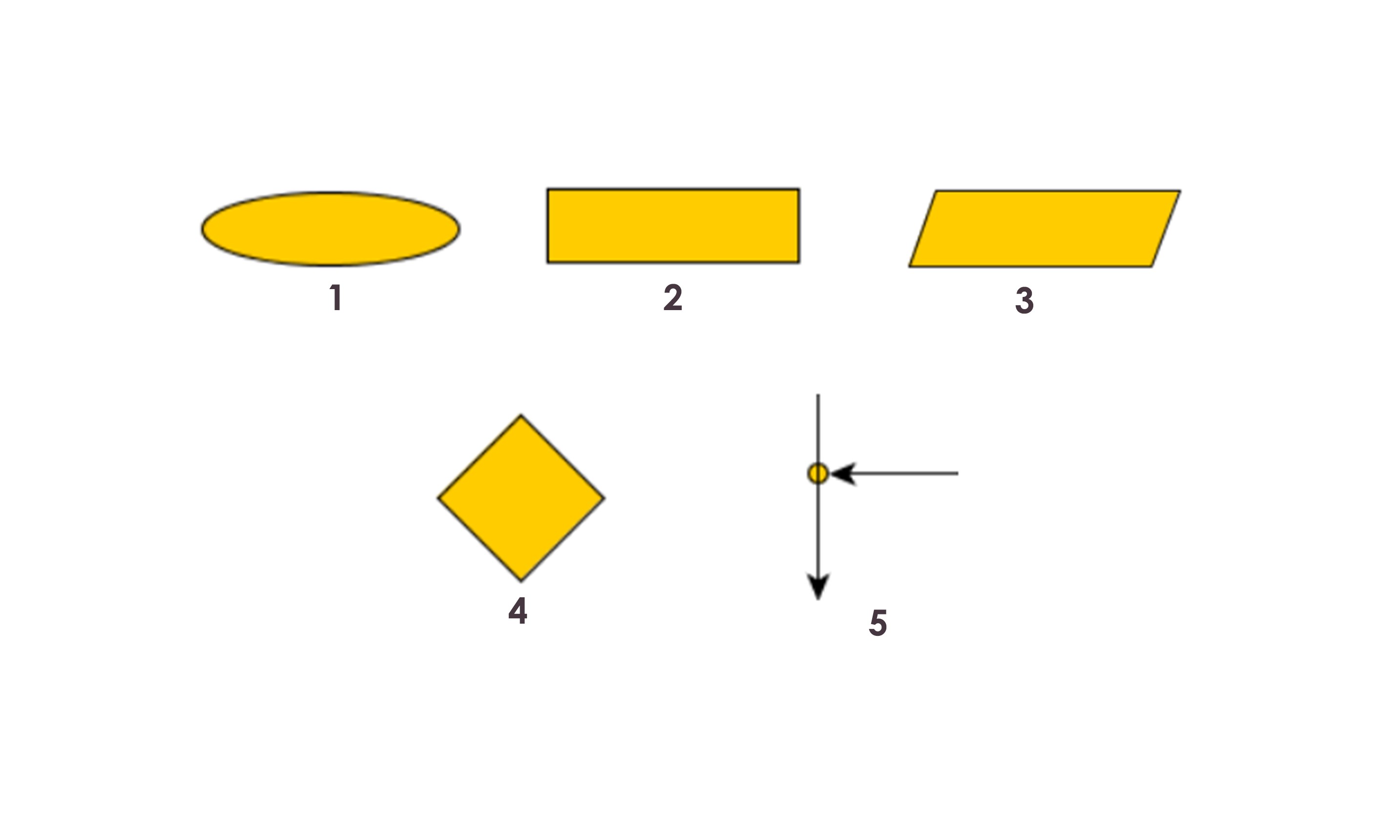
4.This is what we use when our program has to make a decision. This is the only block that has more than one exit arrow. The rhombus symbol has one(or several) entrance points and exactly two outputs.
5.Junction flow chart symbol : You can connect two arrows with a junction
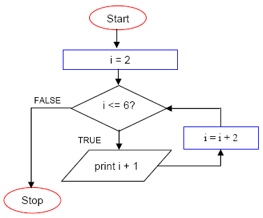
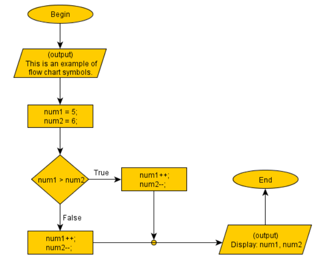
Here are examples of a short algorithm, using each flowcharts
Datatypes

VARIABLES
A variable is a container (storage area) used to hold data.
Each variable should be given a unique name (identifier).
int a=2;
Here a is the variable name that holds the integer value 2.
The value of a can be changed, hence the name variable.
There are certain rules for naming a variable in C++
1. Can only have alphabets, numbers and underscore.
2. Cannot begin with a number.
3. Cannot begin with an uppercase character.
4. Cannot be a keyword defined in C++ language (like int is a keyword).
FUNDAMENTAL DATATYPES IN C++ :
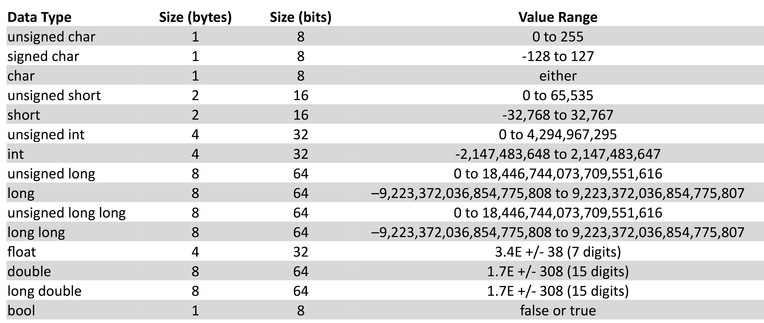
Data types are declarations for variables. This determines the type and size of
data associated with variables which is essential to know since different data
types occupy different size of memory.
1. int:
● This data type is used to store integers.
● It occupies 4 bytes in memory.
● It can store values from -2147483648 to 2147483647.
Eg. int age = 18
2. float and double:
● Used to store floating-point numbers (decimals and exponentials)
● Size of float is 4 bytes and size of double is 8 bytes.
● Float is used to store upto 7 decimal digits whereas double is used to store upto 15 decimal digits.
Eg. float pi = 3.14
double distance = 24E8 // 24 x 108
3. char:
● This data type is used to store characters.
● It occupies 1 byte in memory.
● Characters in C++ are enclosed inside single quotes ͚ ͚.
● ASCII code is used to store characters in memory.
Eg͘ char ch с ͚a͖͛
4. bool
● This data type has only 2 values ʹ true and false.
● It occupies 1 byte in memory.
● True is represented as 1 and false as 0.
Eg. bool flag = false
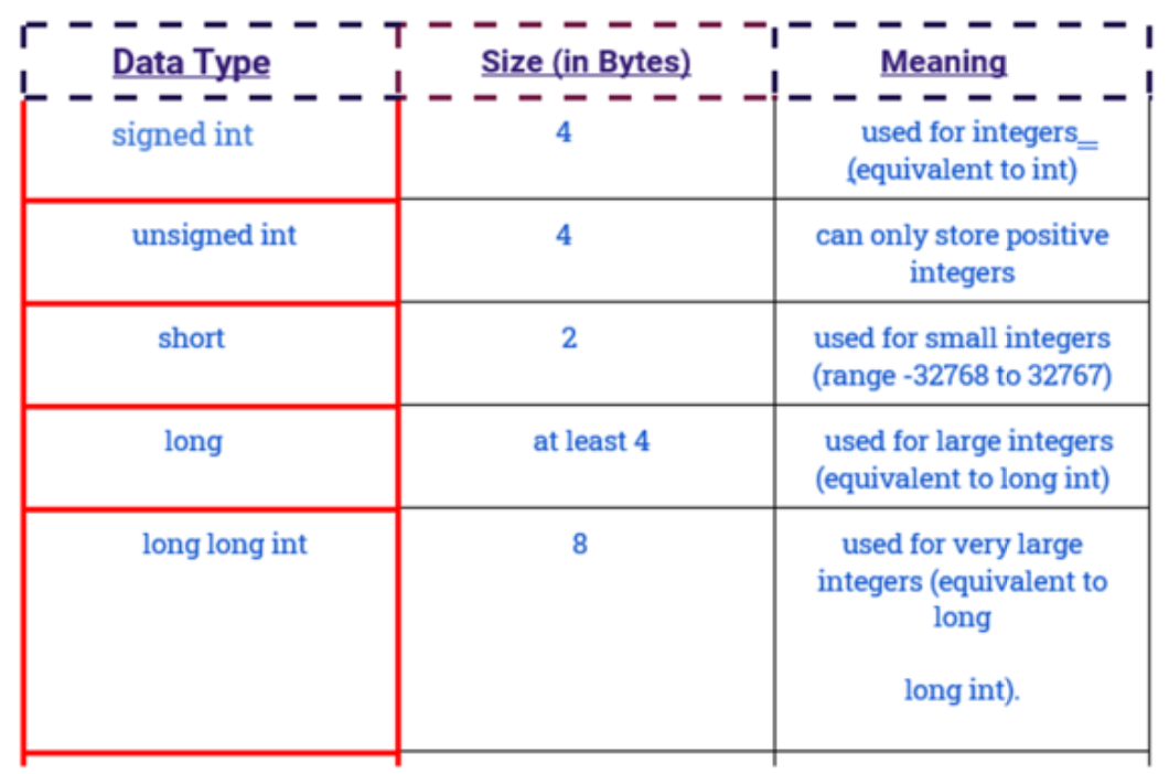
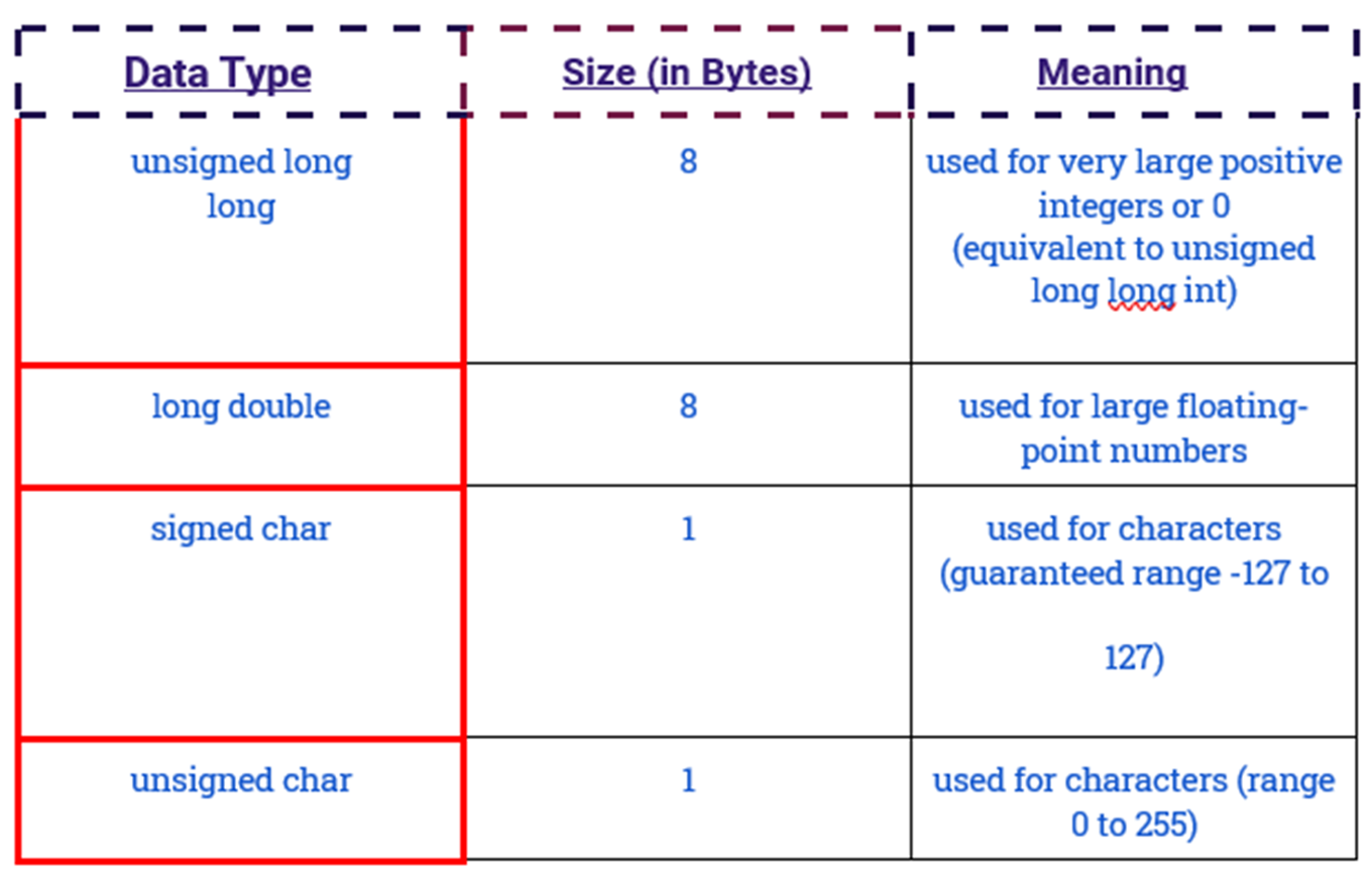
C++ TYPE MODIFIERS
Type modifiers are used to modify the fundamental data types.
DERIVED DATATYPES:
These are the data types that are derived from fundamental (or built-in) data
types. For example, arrays, pointers, function, reference.
USER-DEFINED DATATYPES:
These are the data types that are defined by user itself.For example, class, structure, union, enumeration, etc.
Input/Output
1. Comments
The two slash(//) signs are used to add comments in a program. It does not have any effect on the behavior or outcome of the program. It is used to give a description of the program you’re writing.
2. #include<iostream>
#include is the pre-processor directive that is used to include files in our program. Here we are including the iostream standard file which is necessary for the declarations of basic standard input/output library in C++.
3. Using namespace std
All elements of the standard C++ library are declared within namespace. Here we are using std namespace.
4. int main()
The execution of any C++ program starts with the main function, hence it is necessary to have a main function in your program. ‘int’ is the return value of this function. (We will be studying about functions in more detail later).
5. {}
The curly brackets are used to indicate the starting and ending point of any function. Every opening bracket should have a corresponding closing Bracket.
6. Cout<< ”Hello World!\n”;
This is a C++ statement. cout represents the standard output stream in C++. It is declared in the iostream standard file within the std namespace. The text between quotations will be printed on the screen. \n will not be printed, it is used to add line break. Each statement in C++ ends with a semicolon (;)
7. return 0;
return signifies the end of a function. Here the function is main, so when we hit return 0, it exits the program. We are returning 0 because we mentioned the return type of main function as integer (int main). A zero indicates that everything went fine and a one indicates that something has gone wrong.
                                                        // Hello world program in C++
#include<iostream>
using namespace std;
int main()
{
      cout << "Hello World!\n";
      return 0;
}
Operators in C++
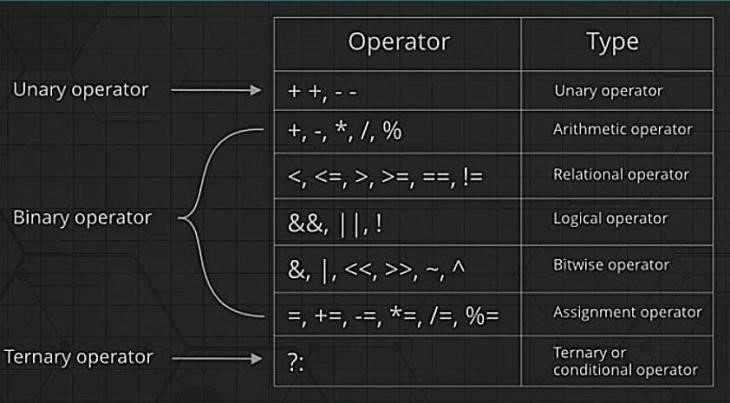
Operators are nothing but symbols that tell the compiler to perform some specific operations. Operators are of the following types -
1. Arithmetic Operators
Arithmetic operators perform some arithmetic operation on one or two operands. Operators that operate on one operand are called unary arithmetic operators and operators that operate on two operands are called binary arithmetic operators. +,-,*,/,% are binary operators. ++, -- are unary operators.
Suppose : A=5 and B=10
Operator Operation Example
+ Adds two operands A+B = 15
- Subtracts right operand from left operand B-A = 5
* Multiplies two operands A*B = 50
/ Divides left operand by right operand B/A = 2
% Finds the remainder after integer division B%A = 0
Pre-incrementer : It increments the value of the operand instantly.
Post-incrementer : It stores the current value of the operand temporarily and only after that statement is completed, the value of the operand is incremented.
Pre-decrementer : It decrements the value of the operand instantly.
Post-decrementer : It stores the current value of the operand temporarily and only after that statement is completed, the value of the operand is decremented.
                                                        int a=10;
int b;
b = a++;
cout<<a<<" "<<b<<endl;
Output : 11 10
int a=10;
int b;
b = ++a;
cout<<a<<" "<<b<<endl;
Output : 11 11
2. Relational Operators
Relational operators define the relation between 2 entities. They give a boolean value as result i.e true or false.
Suppose : A=5 and B=10
Operator Operation Example
== Gives true if two operands are equal A==B is not true
!= Gives true if two operands are not equal A!=B is true
> Gives true if left operand is more than right operand A>B is not true
< Gives true if left operand is less than right operand A<B is true
>= Gives true if left operand is more than right operand or equal to it A>=B is not true
<= Gives true if left operand is more than right operand or equal to it A<=B is true
                                                            int n;
cin>>n;
if(n<10){
     cout<<"Less than 10"<<endl;
}
else if(n==10){
     cout<<"Equal to 10"<<endl;
}
else{
     cout<<"More than 10"<<endl;
}
Example -
We need to write a program which prints if a number is more than 10, equal to 10 or less than 10. This could be done using relational operators with if else statements.
3. Logical Operators
Logical operators are used to connect multiple expressions or conditions together.
We have 3 basic logical operators.
Suppose : A=0 and B=1
&& AND operator. Gives true if both operands are non-zero.(A && B) is false
|| OR operator. Gives true if atleast one of the two operands are non-zero.(A || B) is true
! NOT operator. Reverse the logical state of operand !A is true
Example -
If we need to check whether a number is divisible by both 2 and 3, we will use AND operator
(num%2==0) && num(num%3==0)
If this expression gives true value then that means that num is divisible by both 2 and 3.
(num%2==0) || (num%3==0)
If this expression gives true value then that means that num is divisible by 2 or 3 or both.
4. Bitwise Operators
Bitwise operators are the operators that operate on bits and perform bit-by-bit operations.
Suppose : A=5(0101) and B=6(0110)
& Binary AND. Copies a bit to the result if it exists in both operands.
0101 & 0110 => 0100
| Binary OR. Copies a bit if it exists in either operand.
0101 | 0110 => 0111
^ Binary XOR. Copies the bit if it is set in one operand but not both.
0101^ 0110 => 0011
~ Binary Ones Complement. Flips the bit.
~0101 =>1010
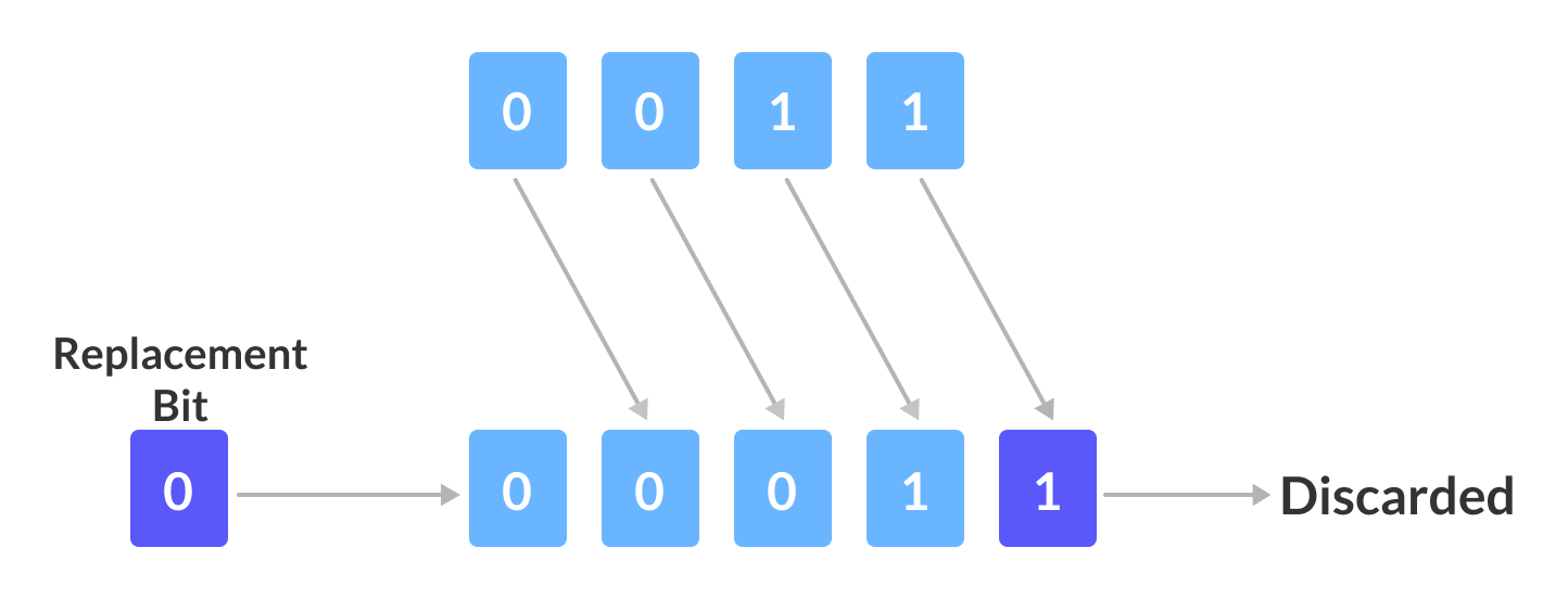
<< Binary Left Shift. Shifts left by the number of places specified by the right operand.
4 (0100)
4<<1=1000 = 8
>> Binary Right Shift. Shifts right by the number of places specified by the right operand.
4>>1=0010 = 2
If shift operator is applied on a number N then,
x N<<a will give a result N*2^a
x N>>a will give a result N/2^a
5. Assignment Operators
= Assigns value of right operand to left operand A=B will put value of B in A
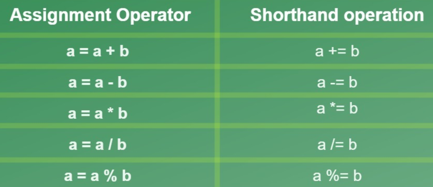
+= Adds right operand to the left operand and assigns the result to left operand.
A+=B means A = A+B
-= Subtracts right operand from the left operand and assigns the result to left operand.
A-=B means A=A-B
*= Multiplies right operand with the left operand and assigns the result to left operand.
A*=B means A=A*B
/= Divides left operand with the right operand and assigns the result to left operand.
A/=B means A=A/B
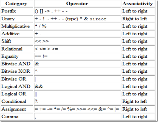
⦿ PRECEDENCE OF OPERATORS
Decision Making
                                                            #include <iostream>
using namespace std ;
int main () {
          int age ;
          cin >> age ;
          if ( age >= 18 ) {
               cout << "You can vote." ;
          }
          else {
          cout << "Not eligible for voting." ;
          }
         return 0 ;
}
IF-ELSE
The if block is used to specify the code to be executed if the condition specified
in it is true, the else block is executed otherwise.
                                                            #include <iostream>
using namespace std ;
int main () {
       int x,y ;
       cin >> x >> y ;
       if ( x == y ) {
            cout << "Both the numbers are equal" ;
       }
       else if ( x > y ) {
            cout << "X is greater than Y" ;
       }
       else {
             cout << "Y is greater than X" ;
        }
        return 0 ;
}
ELSE-IF
To specify multiple if conditions, we first use if and then the consecutive
statements use else if.
                                                            #include <iostream>
using namespace std ;
int main () {
      int x,y ;
      cin >> x >> y ;
      if ( x == y ) {
           cout << "Both the numbers are equal" ;
      }
      else {
           if ( x > y ) {
                    cout << "X is greater than Y" ;
           }
           else {
                    cout << "Y is greater than X" ;
           }
      }
      return 0 ;
}
NESTED-IF
To specify conditions within conditions we make the use of nested ifs.
Loops in C++
                                                            #include<iostream>
using namespace std;
int main(){
     for(int i=1;i<=5;i++){
          cout<<i<<" ";
     }
     return 0;
}
1. for loop:
The syntax of the for loop is
for (initialization; condition; update) {
// body of-loop
}
The for loop is initialized by the value 1, the test condition is i<=5 i.e the loop is
executed till the value of i remains lesser than or equal to 5. In each iteration
the value of i is incremented by one by doing i++.
                                                            #include<iostream>
using namespace std;
int main(){
     int i=1;
     while(i<=5){
          cout<<i<<" ";
          i++;
    }
    return 0;
}
2. while loop
The syntax for while loop is
while (condition) {
// body of the loop
}
The while loop is initialized by the value 1, the test condition is i<=5 i.e the loop
is executed till the value of i remains lesser than or equal to 5. In each iteration
the value of i is incremented by one by doing i++.
                                                            #include<iostream>
using namespace std;
int main(){
     int i=1;
     do
    {
          cout<<i<<" ";
          i++;
     } while (i<=5);
     return 0;
}
3. do͙ while loop
The syntax for while loop is
do {
// body of loop;
}
while (condition);
The do while loop variable is initialized by the value 1, in each iteration the
value of i is incremented by one by doing i++, the test condition is i<=5 i.e the
loop is executed till the value of i remains lesser than or equal to 5. Since the
testing condition is checked only once the loop has already run so a do while
loop runs at least once.
Functions
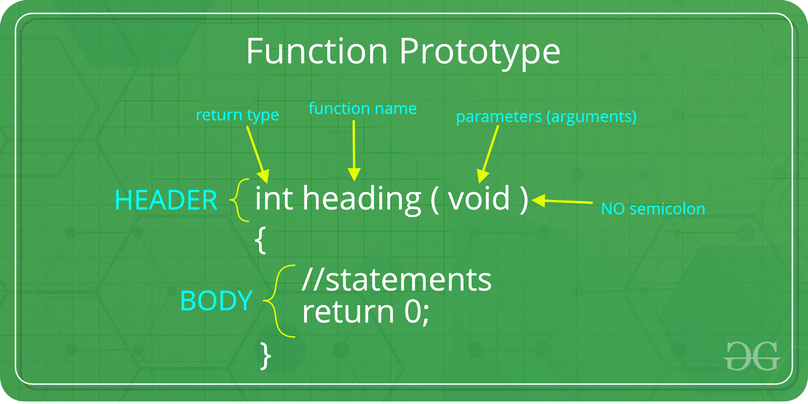
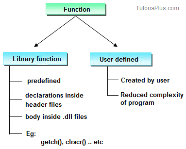
Why are functions used?
x If some functionality is performed at multiple places in software, then rather than writing the same code, again and again, we create a function and call it everywhere. This helps reduce code redundancy. x Functions make maintenance of code easy as we have to change at one place if we make future changes to the functionality. x Functions make the code more readable and easy to understand.
The syntax for function declaration is-
return-type function_name (parameter 1, parameterϮ ...... parameter n){
//function_body
}
return-type
The return type of a function is the data type of the variable that that function returns.
For eg. if we write a function that adds 2 integers and returns their sum then the return type of this function will be ‘int’ as we will returning sum that is an integer value.
When a function does not return any value, in that case the return type of the function is ‘void’.
function_name
It is the unique name of that function. It is always recommended to declare a function before it is used.
Parameters
A function can take some parameters as inputs. These parameters are specified along with their datatypes.
For eg. if we are writing a function to add 2 integers, the parameters would be passed like – int add (int num1, int num2)
Main function:
The main function is a special function as the computer starts running the code from the beginning of the main function. Main function serves as the entry point for the program.
Mathematics
Modular Arithmetic
MODULAR ARITHMETIC
You must have stumbled across problems where you see a large number like 10^9+7 and you tend to skip these ones. After reading this section, handling these would become a cakewalk for you. Let’s start with some basics of modular arithmetic.
INTRODUCTION
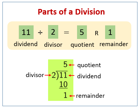
When we divide two integers, we get a quotient Q and a remainder R. To get remainder in programming, we use the modulo operator(%).
Examples:
A % M =R 11 % 2 = 1
13 % 7 = 6
21 % 3 = 0
PROPERTIES
Here are some rules to be followed for performing Modular calculations:
Addition:
(a +b) % m = (a % m + b % m) % m
(6 +8) % 5 = (6 % 5 + 8 % 5) % 5
= (1 + 3) % 5
= 4 % 5
= 4
__________________________________
Subtraction:
(a - b) % m =(a % m - b % m + m) % m
Here, m is added to make the result positive.
(6 - 8) % 5 = (6 % 5 - 8 % 5 +5) % 5
= (1 -3 + 5) % 5 = 3 % 5 = 3
__________________________________
Multiplication:
(a * b) % m = ((a % m) * (b % m)) % m
(6 * 8) % 5 = ((6 % 5) * (8 % 5)) % 5
= (1 * 3) % 5
= 3 % 5
= 3
__________________________________
Division:
Modular division is totally different from modular addition, subtraction and multiplication. It also does not exist always.
(a / b) % m is not equal to ((a % m) / (b % m)) % m
(a / b) % m = ((a % m) * (b^(-1) % m)) % m
Note: b^(-1)is the multiplicative modulo inverse of b and m.
__________________________________
Modular multiplicative inverse:
What is modular multiplicative inverse? If you have two numbers A and M, you are required to find B such it that satisfies the following equation:
(A.B)%M=1
Here B is the modular multiplicative inverse of A under modulo M.
Formally, if you have two integers A and M, B is said to be modular multiplicative inverse of A under modulo M if it satisfies the following equation:
\
A.B≡1(modM) where B is in the range [1,M-1]
Why is B in the range [1,M-1]?

Since we have B%M, the inverse must be in the range [0,M-1]. However, since 0 is invalid, the inverse must be in the range [1,M-1]. An inverse exists only when A and M are coprime i.e. GCD( A ,M )=1.
                                                            int modInverse(int A,int M)
{
    A=A % M;
    for(int B=1;B<M;B++)
        if((A*B) % M)==1)
            return B;
}
Approach 1 (basic approach)
Time Complexity :
The algorithm mentioned above runs in O(M).
                                                            int modInverse(int A,int M)
{
    return modularExponentiation(A,M-2,M);
}
Approach 2 (used only when M is prime)
This approach uses Fermat's Little Theorem.
The theorem specifies the following: ((A)^(M-1)) % M =1
We can divide both sides by A to get : (A^(M-2)) % M = A^(-1)
Yes, we just need A^(M-2). It can be easily calculated by modular exponentiation:
Time complexity:
O(log M)
Study Material for Modular Arithmetic
Inclusion-Exclusion
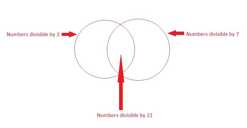
According to inclusion-exclusion principle, to count unique ways for doing a task, the number of ways to do it in one way (n1) and number of ways to do it in some other way (n2) should be added, and the number of ways that are common to both set should be subtracted.
For two finite sets A1 and A2
| A1 ∪ A2 |= |A1 |+ | A2| – |A1 ∩ A2|
Have a look at these examples:
Example 1 :
How many numbers between 10 and 100, including both, have the first digit as 3 and the last digit as 5?
Solution :
The numbers with 1st digit as 3 are from 30,31,32.…..39. So, the number of numbers with 1st digit as 3 is equal to 10. The numbers with last digit as 5 are 15,25,35…..95. Hence, the number of numbers with last digit as 5 is equal to 9.
So, is 10 + 9 = 19 the answer? No.
Because, we haven’t subtracted the common part between the two sets. We need to find the numbers who have both the first digit as 3 and the last digit as 5. Here, there’s only 1 such number, i.e. 35.
Therefore, the final answer = 10 + 9 - 1 = 18.
Example 2 :
How many numbers between 1 and 100, including both, are divisible by 3 and 7?
Solution :
Number of numbers divisible by 3 = 100 / 3 = 33.
Number of numbers divisible by 7 = 100 / 7 = 14.
Number of numbers divisible by 3 and 7 = 100 / (3 * 7) = 100 / 21 = 4.
Hence, number of numbers divisible by 3 or 7 = 33 + 14 - 4 = 43.
If there are more than two sets, the following general formula is applicable:
For a given set A of n sets A_1,A_2,....A_n, let S_nbe the number of ways to do the task :

Here, we can observe that odd number of terms are added while even number of terms are subtracted.
Actually, each subset of is considered exactly once in the formula, thus the formula for a set of n sets has 2^n components.
Problem :
Given two positive integers n and r . Count the number of integers in the interval [1,r] that are relatively prime to n (their GCD is 1).
Solution:
Let’s first find the number of integers between 1 and r that are not relatively prime with n ( i.e they share atleast one prime factor with n ).
So, the first step is to find the prime factors of n. Let the prime factors of n be p_i(i = 1...k )
How many numbers in the interval [1,r] are divisible by p_i? The answer is :

However, if we simply sum these numbers, some numbers will be summarized several times (those that share multiple pias their factors). Therefore, it is necessary to use the inclusion-exclusion principle.
We will iterate over all 2ksubsets of pis, calculate their product and add or subtract the number of multiples of their product.
Below is the C++ implementation of the above idea:
                                                        // CPP program to count the
// number of integers in range
// 1-r that are relatively
// prime to n
#include <bits/stdc++.h>
using namespace std;

// function to count the
// number of integers in range
// 1-r that are relatively
// prime to n
int count (int n, int r) {

    vector<int> p; // vector to store prime factors of n


    // prime factorisation of n
    for (int i=2; i*i<=n; ++i)
        if (n % i == 0) {
            p.push_back (i);
            while (n % i == 0)
                n /= i;
        }
    if (n > 1)
        p.push_back (n);

    int sum = 0;
    for (int mask=1; mask<(1<<p.size()); ++mask) {
        int mult = 1,
            bits = 0;
        for (int i=0; i<(int)p.size(); ++i)
            // Check if ith bit is set in mask
            if (mask & (1<<i)) {
                ++bits;
                mult *= p[i];
            }

        int cur = r / mult;
        if (bits % 2 == 1)
            sum += cur; // if odd number of prime factors are selected
        else
            sum -= cur; // if even number of prime factors are selected

    }

    return r - sum;
}

// Driver Code
int main()
{
    int n=30;
    int r=30;
    cout << count(n, r);
    return 0;
}

//OUTPUT : 22
Study Material for Inclusion-Exclusion
Combinatorics
PERMUTATIONS :
● Permutation: It is the different arrangements of a given number of elements taken one by one, or some, or all at a time.
● For example, if we have two elements A, B and C, then there are 6 possible permutations, ABC, ACB, BAC, BCA, CAB, CBA.
Basic Formula for permuting r items from a collection of n items is represented in mathematics by nPr. The mathematical formula for the same is:
Formula for Permutations of r elements of n elements:
Permutations with repetitions :
If we have n objects, p1 of one kind, p2 of another kind, p3 are another kind and rest are different.
Then the number of permutations for this condition are,
Permutations = n! / (p1! + p2! + p3! + …)
Circular Permutations :
Circular permutation is the total number of ways in which n distinct objects can be arranged around a fix circle. It is of two types:
Clockwise and Anticlockwise orders are different:
Permutations = (n−1)!
Clockwise and Anticlockwise orders are same.
Permutations = (n−1)!/2!
COMBINATIONS :
● Combination: It is the different selections of a given number of elements taken one by one, or some, or all at a time.
● For example, if we have two elements A and B, then there is only one way select two items, we select both of them.
Basic Formula for selecting r items from a collection of n items is represented in mathematics by nCr. The mathematical formula for the same is:
Remember in combination the order of the combination does not matter at all. It is more about the distinct items we are choosing from the set of given items (there is no repetition here in the n items as of now
Here are some useful formulas to use in combination:
● nCr = nCn-r
● nCn = nC0 = 1
Useful Links Combinatorics
Probability
As we all know by now, Probability is how likely something is about to happen.
Let’s denote an event by A, for which we need to find the probability of how likely the event is going to happen. We denote this by using P(A).
And mathematically, P(A) = Number of outcomes where A happens / Total outcomes.
Basic probability calculations
Complement of A : Complement of an event A means not A. Probability of complement event of A means the probability of all the outcomes in sample space other than the ones in A.
P(Ac) = 1 − P(A).
Union and Intersection : The probability of intersection of two events A and B is P(A∩B). When event A occurs in union with event B then the probability together is defined as P(A∪B) = P(A) + P(B) − P(A∩B) which is also known as the addition rule of probability.
Mutually exclusive : Any two events are mutually exclusive when they have non-overlapping outcomes i.e. if A and B are two mutually exclusive events then, P(A∩B) = 0. From the addition rule of probability
P(A∪B) = P(A) + P(B)
as A and B are disjoint or mutually exclusive events.
Independent : Any two events are independent of each other if one has zero effect on the other i.e. the occurrence of one event does not affect the occurrence of the other. If A and B are two independent events then, P(A∩B) = P(A) ∗ P(B).
Conditional Probability
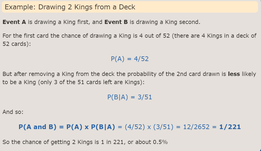
The conditional probability of an event B is the probability that the event will occur given the knowledge that an event A has already occurred. This probability is written P(B|A), notation for the probability of B given A. In the case where events A and B are independent (where event A has no effect on the probability of event B), the conditional probability of event B given event A is simply the probability of event B, that is P(B).
If events A and B are not independent, then the probability of the intersection of A and B (the probability that both events occur) is defined by P(A and B) = P(A)P(B|A).
From this definition, the conditional probability P(B|A) is easily obtained by dividing by P(A):
Binomial Distribution
To get started first we need to learn about something called Bernoulli Trial. Bernoulli Trial is a random experiment with only two possible, mutually exclusive outcomes. And each Bernoulli Trial is independent of the other.
To better understand stuff, let’s see an example.
Suppose we toss a fair coin three times. And we need to find the probability of two heads in all the possible outcomes.
Now, we can see that the probability of getting heads is ½, and tails is also ½, for a fair coin. And here all the tosses of the coin are independent to each other. So, we may say that the single tossing of the coin is a Bernoulli Trial, with the two possible outcomes of heads and tails. Let p denote the probability of getting heads in a fair coin toss. And the other possibility of getting tails is denoted by q. We can see that, p = ½ and q = ½.
The coin is tossed three times, so we have to select two events out of three, where heads will occur. And the total events are three. So, the number of ways to select them is 3C2. And the so can denote the total probability as = 3C2 p2q
Now let’s generalise the approach to problems like these involving Bernoulli Trials.
We saw that the Bernoulli Trial involves two mutually exclusive outcomes. Now for convenience they are often labelled as, “success” and “failure”. The binomial distribution is used to obtain the probability of observing x successes in N trials, with the probability of success on a single trial denoted by p. The binomial distribution assumes that p is fixed for all trials.
Study Material for Probability
LEVEL-1: INITIATED
Number Theory
GCD
GCD(Greatest Common Divisor) or HCF(Highest Common Factor) of 2 integers a and b refers to the greatest possible integer which divides both a and b.
GCD plays a very important part in solving several types of problems(both easy and difficult) which makes it a very important topic for Competitive Programming.
Algorithms to find GCD:
Brute Force Approach:
An approach is possible to start from the smaller number and iterate to 1. As soon as we find a number that divides both a and b, we can return it as the result.
Time complexity: O(min(a,b))
Space complexity: O(1)
Euclidean Algorithm:
The Euclidean Algorithm for calculating the GCD of two numbers builds on several facts:
If we subtract the smaller number from the larger number then the GCD is not changed.
i.e,gcd(a,b)=gcd(b,a-b)[considering a>=b]
If a is 0 and b is non-zero, the GCD is by definition b(or vice versa). If both are zero, then the GCD is undefined; but we can consider it to be zero, which gives us a very basic rule:
If one of the numbers is 0, then the GCD is the other number.
We can build upon these facts and further define GCD as(since the algorithm terminates as soon as one of the numbers become 0):
gcd(a,b)=gcd(b,a%b)
                                                            //Recursive approach
int gcd_recursive (int a, int b) {
    if (b == 0)
        return a;  //if one term is 0, then the  other one is GCD
    else
        return gcd_recursive (b, a % b);
}

//Iterative Approach
int gcd_iterative (int a, int b) {
    while (b) {  //loop continues until b is non-zero
        a %= b;
        swap(a, b);
    }
    return a;
}
Time complexity: O(log(min(a,b)))
Space complexity(Iterative): O(1)
Space complexity(Recursive): O(log(min(a,b))) [Stack space required for recursive function calls]
L.C.M:
LCM (Least Common Multiple) of 2 integers u and v refers to the smallest possible integer which is divisible by both u and v.
                                                            //function to calculate lcm
int lcm (int a, int b) {
    return a / gcd(a, b) * b;
}
LCM also has a very interesting relation with GCD:
u*v=lcm(u,v)*gcd(u*v)
or, lcm(u,v)=(u*v)/gcd(u,v)
[provided u and v both are not zero]
Important Properties:
1. gcd(a,b)=gcd(b,a)
2. gcd(a,b,c)=gcd(a,gcd(b,c))=gcd(gcd(a,b),c)=gcd(b,gcd(a,c))
3. Depending on the parity of a and b, the following cases may arise:
(a). If both the numbers are even, then we can say,
gcd(2*a,2*b)=2*gcd(a,b)
(b). If only one of the numbers is even, while the other is odd,
gcd(2*a,b)=gcd(a,b) [b is odd]
(c). If both numbers are odd,
gcd(a,b)=gcd(b,a−b) [provided a>=b]
Extended Euclidean Algorithm:
The Extended Euclidean Algorithm allows us to find a linear combination of a and b which results in the GCD to a and b.
i,e, a*x+b*y=gcd(a,b) [x,y are integer coefficients]
e.g, a=15, b=35
Therefore,
gcd(a,b)=5
x=-2
y=1
Since, 15*(-2)+35*1=5
Another important topic, Linear Diophantine Equations, will also build upon this algorithm.
Algorithm:
The key factor in understanding the algorithm is figuring out how the coefficients (x,y) change during the change from the function call of gcd(a,b) to gcd(b,a%b) [i.e, following the recursive implementation].
Let us assume we have the coefficients (x1,y1) for (b,a%b);
∴ b*x1+(a%b)*y1=gcd(b,a%b)........(i)
We finally want to find the pair (x,y) for (a,b);
∴ a*x+b*y=gcd(a,b)........(ii)
Again, we know from the rules of modulus:
a%b=a-floor(a/b)*b........(iii)
[floor() function represents the mathematical floor function]
Therefore from equations (i),(ii) and (iii), we can say:
x=y1
y=x1-y1*floor(a/b)
                                                        //Recursive implementation
int extended_euclid_recursive(int a, int b, int& x, int& y) {
    if (b == 0) {
        x = 1;
        y = 0;
        return a;
    }
    int x1, y1;
    int gcd = extended_euclid_recursive(b, a % b, x1, y1);
    x = y1;
    y = x1 - y1 * (a / b);
    return gcd;
}

//Iterative implementation
int extended_euclid_iterative(int a, int b, int& x, int& y) {
    x = 1, y = 0;
    int x1 = 0, y1 = 1, a1 = a, b1 = b;
    while (b1) {
        int q = a1 / b1;
        tie(x, x1) = make_tuple(x1, x - q * x1);
        tie(y, y1) = make_tuple(y1, y - q * y1);
        tie(a1, b1) = make_tuple(b1, a1 - q * b1);
    }
    return a1;
}
Study Material for GCD
Sieve
What is Sieve:
Sieve of Eratosthenes is an algorithm for finding all the prime numbers in a segment in range 1 to n in
0(n log(log n)) operations
Native approach:
                                                            #include <bits/stdc++.h>
using namespace std;
int main()
{
	int n,flag=0;
	cin>>n;
	vector<int> primes;
	for(int i=2;i<=n;i++)
	{
		flag=0;
		for(int j=2;j<i;j++)
		if(i%j==0)
		{
			flag=1;
			break;
		}
		if(flag==0)primes.push_back(i);
	}
	for(int i=0;i<primes.size();i++)cout<<primes[i]<<endl;
}
we iterate the loop from 1 to n and for each number, we check whether it is prime or not.
The time complexity is 0(n*n)
                                                            #include <bits/stdc++.h>
using namespace std;
int main()
{
	int n,flag=0;
	cin>>n;
	vector<int> primes;
	for(int i=2;i<=n;i++)
	{
		flag=0;
		for(int j=2;j*j<=i;j++)
		if(i%j==0)
		{
			flag=1;
			break;
		}
		if(flag==0)primes.push_back(i);
	}
	for(int i=0;i<primes.size();i++)cout<<primes[i]<<endl;

}
A better approach of the above solution:
We can check the divisors up to sqrt(i) since one of the divisors will be smaller than or equal to sqrt(i).
The time complexity of the code is 0(n*sqrt(n))
USING SIEVE:
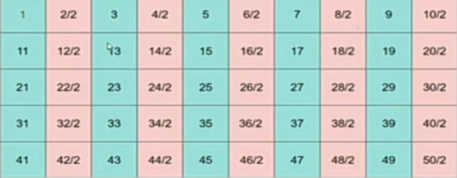
In the sieve algorithm, we create an integer array of length n+1(for numbers from 1 to n) and mark all of them as prime. Then we iterate from 2 till square root of n. We mark all proper multiples of 2 (since 2 is the smallest prime number) as composite. A proper multiple of a number num is a number greater than num and divisible by num. Then we find the next number that hasn't been marked as composite, in this case, it is 3. This means 3 is prime, and we mark all proper multiples of 3 as composite and we continue this procedure.
For n=50, this is the list of primes we are going to get

                                                        #include <bits/stdc++.h>
using namespace std;
int main()
{
	int n;
	cin>>n;
	vector<int> prime(n+1, 1);
	prime[0] = prime[1] = 0;
	for (int i = 2; i * i <= n; i++) {
    	if (prime[i]==1) {
        	for (int j = i * i; j <= n; j += i)
            	prime[j] = 0;
    	}
	}
	for(int i=1;i<=n;i++)if(prime[i]==1)cout<<i<<endl;
}
The time complexity of the above code is 0(n*log(log n))
In the above code, we can reduce the number of operations performed by the algorithm by stopping checking for even numbers as all even numbers (except 2) are composite numbers for we can check for odd numbers only.
                                                        #include <bits/stdc++.h>
using namespace std;
int main()
{
	int n;
	cin>>n;
	vector<int> prime(n+1, 1);
	prime[0] = prime[1] = 0;
	for (int i = 3; i * i <= n; i+=2) {
    	if (prime[i]==1) {
        	for (int j = i * i; j <= n; j += i)
            	prime[j] = 0;
    	}
	}
	if(n>=2)
	cout<<2<<endl;//as 2 is a prime number
	for(int i=3;i<=n;i+=2)if(prime[i]==1)cout<<i<<endl;
}
PRIME FACTORIZATION USING SIEVE:
For finding the prime factors of numbers using sieve first we generate an array and initialize elements with their position, then we perform sieve operation; we mark all the multiples of 2 as 2, multiples of 3 as 3, and so on.
Then for finding prime factors we simply run a loop till n is greater than equal to 1, print the factor stored in ar[n], and then divide n by ar[n].


                                                        #include<bits/stdc++.h>
using namespace std;
vector<int>ar(100000,0);
void sieve(int maxn)
{
	for(int i=0;i<=maxn;i++)ar[i]=i;
	for(int i=2;i*i<=maxn;i++)
	{
		if(ar[i]==i)
		{
			for(int j=i*i;j<=maxn;j+=i)
				ar[j]=i;}
	}
}
int main()
{	sieve(100000);
	int t;
	cin>>t;
	while(t--)
	{	int n;
		cin>>n;
		while(n>=1)
		{	cout<<ar[n]<<endl;
			if(n==1)break;
			n/=ar[n];
		}
	}
}
SEGMENTED SIEVE
The idea of a segmented sieve is to divide the range [0..n-1] in different segments and compute primes in all segments one by one. This algorithm first uses Simple Sieve to find primes smaller than or equal to √(n). Below are steps used in Segmented Sieve.
1. Use Simple Sieve to find all primes up to the square root of ‘n’ and store these primes in an array “prime[]”. Store the found primes in an array ‘prime[]’.
2. we need to find all prime numbers in a range [L, R] of small size (e.g., R−L+1≈1e7), where R can be very large (e.g.10^12)
To solve such a problem, we can use the idea of the Segmented sieve. We pre-generate all prime numbers up to sqrt(R) and use those primes to mark all composite numbers in the segment [L, R].
                                                        vector<bool> segmentedSieve(long long L, long long R) { // generate all primes up to sqrt(R)
long long lim = sqrt(R);
vector<bool> mark(lim + 1, false);
vector<long long> primes;
for (long long i = 2; i <= lim; ++i) {
if (!mark[i]) {
primes.emplace_back(i);
for (long long j = i * i; j <= lim; j += i)
mark[j] = true;
}
}
vector<bool> isPrime(R - L + 1, true);
for (long long i : primes)
for (long long j = max(i * i, (L + i - 1) / i * i); j <= R; j += i)
isPrime[j - L] = false;
if (L == 1)
isPrime[0] = false;
return isPrime;
}

//Time complexity of this approach is O((R-L+1)loglog(R)+sqrt(R)loglog(sqrt(R)))
Study Material for Sieve
LDE
Linear Diophantine Equations
Introduction:
A General Diophantine equation is a polynomial equation, having two(or more) integral variables i.e. if a solution of the equation exists, it possesses integral values.
A linear Diophantine equation is a Diophantine equation of degree 1 i.e. each integral variable in the equation is either of degree 0 or degree 1.
General form:
A Linear Diophantine Equation(in two variables) is an equation of the general form:
ax + by = c
Where a,b,c are integral constants and x,y are integral variables.
Homogeneous Linear Diophantine equation:
A Homogeneous Linear Diophantine Equation(in two variables) is an equation of the general form:
ax + by = 0
Where a,b are integral constants and x,y are the integral variables.
By looking at the equation we can easily observe that x=0 and y=0 is a solution to the equation. This is called the Trivial solution.
Though more solutions can exist for the same.
Condition for the solution to exist:
For a linear diophantine equation, the integral solution exists if and only if:
c%gcd(a,b)=0
i.e. c must be divisible by the greatest common divisor of a and b. This is because
Let, a = gcd(a,b).A, where A is an integral divisor of a. Similarly, b = gcd(a,b).B.
Therefore the Linear Diophantine equation can be written as:
gcd(a,b).A + gcd(a,b).B = c
gcd(a,b).(A + B) = c
This means that c must be a multiple of gcd(a,b).
For the Homogeneous Linear Diophantine equation, a solution always exists i.e. the trivial solution.This is because c=0, and we know 0 is divisible by every integer.
Finding a solution:
A solution can easily be found using the Extended Euclidean algorithm.
.
ax1 + by1 = gcd(a,b)
a.x1.c + by1.c = gcd(a,b).c (multiplying both sides by c)
a.x1.{c/gcd(a,b)} + by1.{c/gcd(a,b)} = c
a.{x1.(c/gcd(a,b))} + b.{y1.(c/gcd(a,b))} = c ….. (1)
Now, by comparing the equation (1) with the general Linear Diophantine equation we get:
x0 = x1 . c/gcd(a,b)
y0 = y1 . c/gcd(a,b)
Where x0 and y0 is a solution of the Linear Diophantine equation.
Implementation:
Program to find a solution of a given Linear Diophantine equation.
                                                        #include<bits/stdc++.h>
using namespace std;
// function to find the gcd of a,b and coefficient x,y
//using Extended Euclidean Algorithm
int extended_gcd(int a, int b, int &x, int &y)
{
	if(a == 0)// base case
	{
		x = 0;
		y = 1;
		return b;// here b will be the gcd.
	}
	int x1, y1;
	int g = extended_gcd(b%a, a, x1, y1);
	x = y1 - (b/a) * x1;
	y = x1;
	return g;
}
// function to find a solution of the Diophantine equation if any
int one_solution(int a, int b, int c, int &x, int &y)
{
   int g = extended_gcd(a, b, x, y);
   if(c%g == 0) // condition for a solution to exist
   {
   	  //solution to the Diophantine equation
   	  x = x * c/g;
   	  y = y * c/g;
   	  return 1;  // Atleast 1 solution exist
   }
   return 0;   // no solution exists
}

int main()
{
   int a,b,c,x,y;
   cin>>a>>b>>c;
   if(one_solution(a,b,c,x,y))// if solution exists
   {
   	 cout<< "Solution are: "
   	 cout<<x<< " "<<y;
   }
   else// if no solution exists
   {
   	cout<< "Solution does not Exist";
   }
}
Time Complexity - O(log(max(a,b)))
Auxiliary Space - O(1)
Finding all solutions:
Let, C0 be any arbitrary integer.
Add and subtract {C0.a.b/gcd(a,b)} in the general Linear Diophantine equation we get,
a.x0 + b.y0 + C0.a.b/gcd(a,b) - C0.a.b/gcd(a,b) = c
(Where x0 and y0 is a solution of the Linear Diophantine)
a.x0 + C0.a.b/gcd(a,b)+ b.y0 - C0.a.b/gcd(a,b) = c
a.(x0 + C0.b/gcd(a,b)) + b.(y0 - C0.a/gcd(a,b)) = c ….. (2)
Comparing equation (2) with general equation of Linear Diophantine equation
we get,
x = x0 + C0.b/gcd(a,b)
y = y0 - C0.a/gcd(a,b)
Where x,y are the solutions of the Linear Diophantine equation.
Study Material for LDE
Reference Study - CP-Algorithms
Diophantine_equation - Wikipedia
Linear-Diophantine-Equations GFG
Linear-Diophantine-Equations-one-equation Brilliant
CRT
Chinese Remainder Theorem
Introduction:
Given set of n equations:
x % q[1] = r[1] or x ≡ r[1] (mod q[1])
x % q[2] = r[2]
x % q[3] = r[3]
.
.
.
x % q[n] = r[n]
Where, q[1], q[2]... q[n] are pairwise coprime positive integers i.e, for any 2 numbers q[i] and q[j] (i≠j)
GCD(q[i] , q[j]) = 1
And r[1].. r[n] are remainders when x is divided by q[1]... q[n] respectively .So, according to the Chinese Remainder theorem, there always exists a solution of a given set of equations and the solution is always unique modulo N, where
N = q[1].q[2]...q[n]
Finding solution:
Assume, C0 be a solution to the set of equations i.e C0 satisfies each and every equation belonging to the set. Then Xi = C0 ± K is also a solution to the set of equations if
K = LCM(q[1],q[2],q[3]....q[n]
LCM denotes the least common multiple of q[1] ,q[2]... q[n].
But ,we know that q[1] ,q[2]...q[n] are pairwise coprime therefore,
LCM(q[1],q[2]...q[n]) = q[1].q[2].q[3]...q[n]
Therefore, positive solutions to the set of equations are
Xi = C0 + K
Where C0 is the minimum positive solution that exists. So to find the solutions of the given set of equations we just need to find the minimum positive solution that exists.
Finding minimum positive solution:
Brute Force Approach:
A simple solution to find the minimum positive solution is to iterate from 1 till we find first value C0 such that all n equations are satisfied.
Implementation: function to find minimum positive solution.
                                                        int Find_x(int q[] ,int r[] ,int n)
{
    int x=1;// initializing minimum positive solution
    bool flag;
    while(1)// we iterate till we get a solution
    {
        flag=true;
        for(int i=0;i<n;i++)
        {
           if(x % q[i] == r[i] )//check if x gives remainder r[i] when divided by q[i]
             continue;
           flag=false;// if remainder is not r[i], this x cannot be the answer
           break;
        }
        if(flag) // if x satisfies all n equations ,then we have found the answer.
          break;
        x++; // check for further values
    }
    return x;
}
Efficient Approach:
The general solution of the set of equation looks like
Xi = r[1].y[1].inv[1] + r[2].y[2].inv[2] . . . . . r[n].y[n].inv[n] .... (1)
Where,
y[1] = q[2].q[3].q[4]....q[n] or y[1] = N/q[1]
y[2] = q[1].q[3].q[4]....q[n]
.
.
.
y[n] = q[1].q[2].q[3].....q[n-1]
and,
inv[1] = y[1]-1 mod q[1]
inv[2] = y[2]-1 mod q[2]
.
.
.
inv[n] = y[n]-1 mod q[n]
We, know that the Chinese Remainder theorem states that there always exists a solution and this solution is always unique modulo N.So, to find the minimum positive solution we take (Xi mod N) where N = q[1].q[2]....q[n]. Therefore
x = Xi %N or
x = (r[1].y[1].inv[1] + r[2].y[2].inv[2] . . . . . r[n].y[n].inv[n]) % N …. (2)
Implementation: function to find minimum positive solution.
                                                        // function to find gcd and coefficients using Extended Euclidean Algorithm
int Extended_gcd(int a ,int b, int &x, int &y)
{
    if(a==0)
    {
        x = 0;
        y = 1;
        return b;
    }
    int x1 ,y1;
    int g = Extended_gcd(b % a, a, x1, y1);
    x = y1 - (b / a) * x1;
    y = x1;
    return g;
}
//function to find inverse of val w.r.t m
int inv(int val ,int m)
{
    int x ,y;
    int g = Extended_gcd(val ,m ,x ,y);
    if(x < 0)
        x = (x % m + m) % m;
    return x;
}
int Find_x(int q[] ,int r[] ,int n) //function to find minimum positive solution
{
    int x=0 ,N=1;
    for(int i=0;i<n;i++)
        N *= q[i]; // compute N = q[0].q[1]..q[n-1]
    for(int i=0;i<n;i++)
    {
       int y = N / q[i];
       x = ( x + r[i] * y * inv(y ,q[i]) ) % N; //computing x according to equation 2
    }
    return x;
}
Study Material for CRT
Chinese Remainder Theorem - cp-algorithms reference
Chinese Remainder Theorem - Wikipedia Reference
Chinese Remainder Theorem - GFG
Chinese Remainder Theorem - Codechef
Chinese Remainder Theorem - Youtube reference
Practice Problem 1
Practice Problem 2
Practice Problem 3
Fermat's Theorem
FERMAT’S LITTLE THEOREM
Fermat’s little theorem states that if p is a prime number, then for any integer a, the number ap – a is an integer multiple of p.
ap ≡ a (mod p), where p is prime.
If a is not divisible by p, Fermat’s little theorem is equivalent to the statement that ap-1 -1 is an integer multiple of p.
ap - 1 ≡ 1 (mod p)
1. Applications of Fermat’s little theorem
Modular multiplicative Inverse
If we know p is prime, then we can also use Fermats’s little theorem to find the inverse.
ap-1 ≡ 1 (mod p)
If we multiply both sides with a-1, we get
a-1 ≡ a p-2 (mod p)
                                                        // C++ program to find modular multiplicative inverse
//using fermat's little theorem.
#include <bits/stdc++.h>
using namespace std;

// Modular Exponentiation to compute x^y under modulo p
int power(int x, unsigned int y, unsigned int p)
{
    if (y == 0)
        return 1;
    int res = power(x, y / 2, p) % p;
    res = (res * res) % p;

    return (y % 2 == 0) ? res : (x * res) % p;
}

// Function to find modular inverse of a under modulo p
void modInverse(int a, int p)
{
    if (__gcd(a, p) != 1)
        cout << "Inverse doesn't exist";
    else {
        // If a and p are relatively prime, then
        // modulo inverse is a^(p-2) mode p
        cout << "Modular multiplicative inverse is "
            << power(a, p - 2, p);
    }
}

// Driver Program
int main()
{
    int a = 3, p = 11;
    modInverse(a, p);
    return 0;
}
2. Primality Test
In Fermat Primality Testing, k random integers are selected as the value of a (where all k integers follow gcd(a,k) = 1). If the statement of Fermat's Little Theorem is accepted for all these k values of a for a given number N, then N is said as a probable prime.
                                                        // C++ program to check if N is prime.
#include <bits/stdc++.h>
using namespace std;

/* Iterative Function to calculate (a^n)%p in O(logy) */
int power(int a, unsigned int n, int p)
{
    int res = 1; // Initialize result
    a = a % p; // Update 'a' if 'a' >= p

    while (n > 0)
    {
        // If n is odd, multiply 'a' with result
        if (n & 1)
            res = (res*a) % p;

        // n must be even now
        n = n>>1; // n = n/2
        a = (a*a) % p;
    }
    return res;
}

// If n is prime, then always returns true, If n is
// composite then returns false with high probability
// Higher value of k increases probability of correct
// result.
bool isPrime(unsigned int n, int k)
{
    // Corner cases
    if (n <= 1 || n == 4) return false;
    if (n <= 3) return true;

    // Try k times
    while (k>0)
    {
        // Pick a random number in [2..n-2]
        // Above corner cases make sure that n > 4
        int a = 2 + rand()%(n-4);

        // Checking if a and n are co-prime
        if (__gcd((int)n, a) != 1)
            return false;

        // Fermat's little theorem
        if (power(a, n-1, n) != 1)
            return false;

        k--;
    }

    return true;
}

// Driver Program to test above function
int main()
{
    int k = 3;
    isPrime(11, k)? cout << " true\n": cout << " false\n";
    isPrime(15, k)? cout << " true\n": cout << " false\n";
    return 0;
}
Study Material for Fermat's Theorem
Compute nCr % p - Using Fermat's Theorem
GFG - Fermat's Little Theorem
Practice Problem 1
Practice Problem 2
Bitwise
Operations and Properties
Introduction to Bits
We usually work with data types such as int, char, float, etc., or even data structures( i.e generally on bytes level) but sometimes programmers need to work at bit level for various purposes such as encryption, data compression, etc.
Apart from that operations on bits are time efficient and are used for optimizing programs.
Bit Manipulation
Any number can be represented bitwise
which is known as its binary form or base-2 form.
1 byte comprises 8 bits.
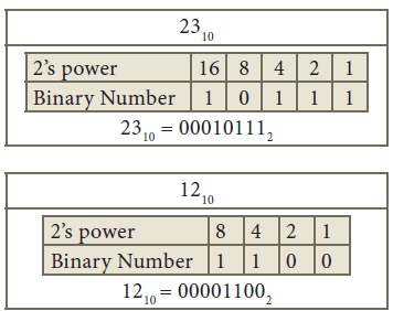
For example:
(21)10 = (10101)2 in binary form.
= 1*24 + 0*23 + 1*22 + 0*21 + 1*20
Suppose we use int to store 21 and we
know int is of 4 bytes so it will be using
32 bit representation with last five bits
as 10101.
Bitwise Operators
There are different operators that work on bits and are used for optimizing programs in terms of time.
Unary Operators
1. NOT (!) : Bitwise NOT is an unary operator that flips the bits of the number i.e., if the bit is 0, it will change it to 1 and vice versa.It gives the one’s complement of a number.
Example: - N = 5 = (101)2
~N = ~5 = ~(101)2 = (010)2 = 2
Binary Operators
1. AND (&) : Bitwise AND operates on two equal-length bit patterns. If both bits at the ith position of the bit patterns are 1, the bit in the resulting bit pattern is 1, otherwise 0.
Example:-
00001100 = (12)10
& 00011001 = (25)10
_________
00001000 = (8)10
2. OR ( | ) : Bitwise OR also operates on two equal-length bit patterns. If both bits at the ith position of the bit patterns are 0, the bit in the resulting bit pattern is 0, otherwise 1.
Example:-
00001100 = (12)10
| 00011001 = (25)10
_________
00011101 = (29)10
3. XOR ( ^ ) : Bitwise XOR also operates on two equal-length bit patterns. If both bits in the ith position of the bit patterns are 0 or 1, the bit in the resulting bit pattern is 0, otherwise 1.
Example:-
00001100 = (12)10
^ 00011001 = (25)10
_________
00010101 = (21)10
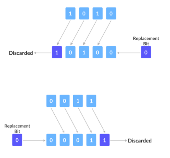
4. Left Shift ( << ): Left shift operator is a binary operator that shifts some number of bits, in the given bit pattern, to the left and appends 0 at the right end. Left shift is equivalent to multiplying the bit pattern with 2k.(say we are shifting bits by k-positions).
Example :-
Consider shifting 8 to the left by 1
(8)10 =(1010)2
5. Right Shift ( >> ): Right shift operator is a binary operator that shifts some number of bits, in the given bit pattern, to the right and appends 0 at the left end. Right shift is equivalent to dividing the bit pattern with 2k ( say we are shifting by k-positions ).
Example:-
Consider shifting 3 to the right by 1
(3)10 = (0011)2
Basics Operations on Bits
                                                            int x = 16;
if ( x & (1 << i) )
{
        // i th bit is set
}
else
{
        // i th bit is not set
}
1. Bitwise ANDing (Masking):- This is used for checking if the ith bit in the given bit pattern is set or not.
Example :-
Let x=12 and we have to check if the 3rd bit is set or not.
                                                            int x = 12;
x = x | (1 <<i );
2. Bitwise ORing:- This is used to set ith bit in the given bit pattern.
Example:-
Let x=12 and we have to set the 1st bit in x.
                                                            int x = 12;
x = x ^ (1 <<i );
3. Bitwise XORing :- This is used to toggle ith bit in the given bit pattern.
Example:-
Let x = 12 and we have to toggle 2nd bit in x.
Tricks with Bits
1. x ^ ( x & (x-1)) : Returns the rightmost 1 in binary representation of x.
(x & (x - 1)) will have all the bits equal to the x except for the rightmost 1 in x. So if we do bitwise XOR of x and (x & (x-1)), it will simply return the rightmost 1. Let’s see an Example:-
x = 10 = (1010)2 `
x & (x-1) = (1010)2 & (1001)2 = (1000)2
x ^ (x & (x-1)) = (1010)2 ^ (1000)2 = (0010)2
2. x & (-x) : Returns the rightmost 1 in binary representation of x
(-x) is the two’s complement of x. (-x) will be equal to one’s complement of x plus 1.
Therefore (-x) will have all the bits flipped that are on the left of the rightmost 1 in x. So x & (-x) will return rightmost 1.
Example:-
x = 10 = (1010)2
(-x) = -10 = (0110)2
x & (-x) = (1010)2 & (0110)2 = (0010)2
3. x | (1 << n) : Returns the number x with the nth bit set.
(1 << n) will return a number with only nth bit set. So if we OR it with x it will set the nth bit of x.
x = 10 = (1010)2 n = 2
1 << n = (0100)2
x | (1 << n) = (1010)2 | (0100)2 = (1110)2
Study Material for Bitwise
LEVEL-2: TRAINED
Searching
Linear Search
In the programming world, we often need to find out whether an element is present in the given data set or not.
Formally, we have an array and we are asked to find the index of an element ‘k’ in the array. And if it is not present, inform that.
The simplest way to answer this question is Linear Search.
In linear search, we traverse the entire array and check each element one by one.
                                                            int flag=0;
for(start to end of the array){
	if(current_element is k){
	      cout<<“Required element is found at”<<current_index<<endl;
	      flag=1;
      break;
}
}
if(flag==0){
	cout<<”Required Element not present in the array”<<endl;
}
As one can easily see, in the worst case i.e. when the element is not present in the array, we are traversing the entire array. Hence the time complexity of this operation is O(n).
Study Material for Linear Search
Binary Search
Binary Search is the most useful search algorithm. It has many applications too, mainly due to its logarithmic time complexity. For example, if there are 109 numbers and you want to search for a particular element, using binary search you can do this task in just around 32 steps!
The only thing that one must keep in mind is that binary search works only on sorted set of elements.
The main idea of the algorithm can be explained as follows:
Let we have a sorted array of n elements, and we want to search for k.
Let's compare k with the middle element of the array.
If k is bigger, it must lie on the right side of the middle element.
Else if it is smaller, it must lie on the left side of the middle element.
This means, in one step, we reduced the “search space” by half. We can continue this halfing-process recursively until we find the required element. That's it.
Remember, we could do this because the elements were sorted.
Here, in each step we half the length of the interval. In the worst case, we continue the process till the length becomes 1. Hence, the time complexity of binary search is O(log2 N), where N is the initial length of interval.
                                                            // Function to find the index of an element k in a sorted array arr.
int binarySearch(int arr[], int l, int r, int k){
    while (l <= r) {
   	 int mid = l + (r - l) / 2;
   	 // Check if x is present at mid
   	 if (arr[mid] == k)
   		 return m;      // Found the element.
   	 // If x greater, ignore left half
   	 if (arr[mid] < k)
   		 l = mid + 1;
   	 // If x is smaller, ignore right half
   	 else
   		 r = mid - 1;
    }
    // if we reach here, then the element was not present.
    return -1;
}
We can implement binary search algorithm either iteratively or recursively.
Iterative Implementation
                                                            int binarySearch(int arr[], int l, int r, int k)
{
    if (r >= l) {
        int mid = l + (r - l) / 2;
        // If the element is present at the middle
        if (arr[mid] == k)
            return mid;
        // If the element is smaller than mid, continue searching in the left half.
        if (arr[mid] > k)
            return binarySearch(arr, l, mid - 1, x);

        // Else continue searching in the right half.
        return binarySearch(arr, mid + 1, r, x);
    }

    // We reach here when an element is not present in the array.
    return -1;
}
Recursive implementation
Sometimes a situation arises where we can’t calculate the answer directly from given data due to too many possibilities, but we can have a way to know if a number is possible as a solution or not. i.e. we ask a number and get a feedback as “yes” or “no”. And using the feedback we shorten our “search space”, and continue the search for our answer.
This technique is known as Binary Search the Answer.
Study Material for Binary Search
Lower Bound and Upper Bound
Lower Bound: Lower bound of a number in a sorted array is the first element in that array that is not smaller than the given number. STL has a useful inbuilt function
lower_bound(start_ptr, end_ptr, num) to carry out this task. It returns the pointer pointing to the required element. As this function uses binary search in its working, its time complexity is O(log n).
Upper Bound: Upper bound of a number in a sorted array is the number that is just higher than the given number. STL provides an inbuilt function for this too:
upper_bound(start_ptr, end_ptr, num). Similar to lower_bound(), this function also returns the pointer pointing to the required element, and its time complexity is O(log n).
Note: These functions return the end pointer if the required element is not present in the array.
Note: If there are multiple occurrences of the required element in the array, these functions return the pointer to the first occurrence of it.
                                                            vector<int> Ar={1,1,2,4,4,5,6,7};
       auto l=lower_bound(Ar.begin(),Ar.end(),4);
     // return pointer to index 3
   auto u=upper_bound(Ar.begin(),Ar.end(),4);
// returns pointer to index 5
   cout<<(*l)<<endl;
   cout<<(*u)<<endl;
Output:
4
5
Study Material for Lower and Upper Bound
Ternary Search
Just like the Binary search algorithm, Ternary search is also a divide and conquer algorithm. And the array needs to be sorted to perform ternary search.The only difference is, instead of dividing the segment into two parts, here we divide it into three parts, and find in which part our key element lies.
1.First, we compare the key with the element at mid1. If found equal, we return mid1.
2.If not, then we compare the key with the element at mid2. If found equal, we return mid2.
3.If not, then we check whether the key is less than the element at mid1. If yes, then recur to the first part.
4.If not, then we check whether the key is greater than the element at mid2. If yes, then recur to the third part.
5.If not, then we recur to the second (middle) part

                                                        int ternary_search(int l,int r, int k)
{
    if(r>=l)
    {
        int mid1 = l + (r-l)/3;
        int mid2 = r -  (r-l)/3;
        if(ar[mid1] == k)
            return mid1;
        if(ar[mid2] == k)
            return mid2;
        if(k<ar[mid1])		 // First part
            return ternary_search(l,mid1-1,k);
        else if(k>ar[mid2])	// Third part
            return ternary_search(mid2+1,r,k);
        else  			// Second part
            return ternary_search(mid1+1,mid2-1,k);
    }
    return -1;
}
Study Material for Ternary Search
Sorting
Selection Sort
The idea behind this algorithm is pretty simple. We divide the array into two parts: sorted and unsorted. The left part is a sorted subarray and the right part is an unsorted subarray. Initially, the sorted subarray is empty and the unsorted array is the complete given array.
We perform the steps given below until the unsorted subarray becomes empty:
(Assuming we want to sort it in non-decreasing order)
Pick the minimum element from the unsorted subarray.
Swap it with the leftmost element of the unsorted subarray.
Now the leftmost element of the unsorted subarray becomes a part (rightmost) of the sorted subarray and will not be a part of the unsorted subarray.
                                                            void selection_sort (int Arr[ ], int n)
         int minimum;    // temporary variable to store the position of minimum element
          // reduces the effective size of the array by one in  each iteration.
         for(int i = 0; i < n-1 ; i++){
               // element at index i will be swapped
  // finding the smallest element of unsorted part:
 	  minimum = i ;
// gives the effective size of the unsorted  array .
 for(int j = i+1; j < n ; j++ ) {
         if(A[ j ] < A[ minimum ])  {
                minimum = j ;
           }
   }
 // putting the minimum element on its proper position.
   swap ( A[ minimum ], A[ i ]) ;
            }
 }
Lets try to understand the algorithm with an example: Arr[ ] = {69, 55, 2, 22, 1}.
At first our array looks like this:{69,55,2,22,1}
Find the minimum element in Arr[0...4] and place it at beginning
{1,55,2,22,69}
Find the minimum element in Arr[1...4] and place it at beginning of Arr[1...4]
{1,2,55,22,69}
Find the minimum element in arr[2...4] and place it at beginning of arr[2...4]
{1,2,22,55,69}
Find the minimum element in arr[3...4] and place it at beginning of arr[3...4]
{1,2,22,55,69}
Time Complexity: O(n2) as there are two nested loops.
Note:
Selection sort never requires more than n swaps.
It is an in-place sorting algorithm.
Its stability depends on implementation.
Study Material for Selection Sort
Bubble Sort
Bubble sort, sometimes referred to as sinking sort, is based on the idea of repeatedly comparing pairs of adjacent elements and then swapping their positions if they exist in the wrong order. In one iteration of the algorithm the smallest/largest element will result at its final place at end/beginning of an array. So in some sense movement of an element in an array during one iteration of bubble sort algorithm is similar to the movement of an air bubble that raises up in the water, hence the name.
Lets try to understand the algorithm with an example: Arr[ ] = {9,2,7,5}.
At first our array looks like this:
{9,2,7,5}
In the first step, we compare the first 2 elements, 2 and 9, As 9>2 , we swap them.
{2,9,7,5}
Next, we compare 9 and 7 and similarly swap them.
{2,7,9,5}
Again, we compare 9 and 5 and swap them.
{2,7,5,9}
Now as we have reached the end of the array, the second iteration starts.
In the first step, we compare 2 and 7. As 7>2, we need not swap them.
{2,7,5,9}
In the Next step, we compare 7 and 5 and swap them.
{2,5,7,9}
In this way, the process continues.
In this example, there will not be any more swaps as the array is sorted after the steps shown above.
                                                            void bubble_sort( int A[ ], int n ) {
    int temp;
    for(int i = 0; i< n-1; i++) {
 // (n-1) because the last element will already be sorted
        for(int j = 0; j < n-i-1; j++) {
//(n-i-1) because remaining i elements are already sorted
            if(A[ j ] > A[ j+1] ){   // here swapping of positions is being done.
                temp = A[ j ];
                A[ j ] = A[ j+1 ];
                A[ j + 1] = temp;
            }
        }
    }
}
Observe that, the above function always runs in O(n2) time even if the array is sorted. It can be optimized by stopping the algorithm if the inner loop didn’t cause any swap.
Note:
>Bubble sort is a stable, in place sorting algorithm.
>Bubble sort does not have any practical application. Yet, it is very much necessary to learn about it as it represents the basic foundations of sorting.
Study Material for Bubble Sort
Insertion Sort
Insertion sort is the sorting mechanism where the sorted array is built having one item at a time. The array elements are compared with each other sequentially and then arranged simultaneously in some particular order. The analogy can be understood from the style we arrange a deck of cards in our hand. This sort works on the principle of inserting an element at a particular position, hence the name Insertion Sort.
To sort an array of size n in ascending order:
1: Iterate from arr[1] to arr[n] over the array.
2: Compare the current element (key) to its predecessor.
3: If the key element is smaller than its predecessor, compare it to the elements before. Move the greater elements one position up to make space for the swapped element.
Lets try to understand the algorithm with an example: Arr[ ] = {69, 55, 2, 22, 1}.
At first our array looks like this:
{69,55,2,22,1}
Let us loop from index 1 to index 4
For index=1, Since 55 is smaller than 69, move 69 and insert 55 before 69
{55,69,2,22,1}
For index=2, 2 is smaller than both 55 and 69. So shift 55 and 69 to right and insert 2 before them.
{2,55,69,22,1}
For index=3, 22 is smaller than both 55 and 69. So shift 55 and 69 to right and insert 22 before them.
{2,22,55,69,1}
For index=4, 22 is smaller than both 55 and 69. So shift 55 and 69 to right and insert 22 before them.
{1,2,22,55,69}
                                                            void insertionSort(int Arr[], int n)
{     int i, key, j;
      for (i = 1; i < n; i++)
      {      key = Arr[i];
               j = i - 1;
           /* Move elements of arr[0..i-1], that are greater than key,
             to one position ahead of their current position */
            while (j >= 0 && Arr[j] > key)
            {     Arr[j + 1] = Arr[j];
                   j = j - 1;
             }
             Arr[j + 1] = key;
      }
 }
me Complexity: O(n2)
Note:
It is an in-place, stable sorting algorithm.
Insertion sort is used when the number of elements is small. It can also be useful when the input array is almost sorted, only a few elements are misplaced in complete big array.
Study Material for Insertion Sort
Merge Sort
Merge sort algorithm works on the principle of Divide and Conquer.
It is one of the most efficient sorting algorithms. It is one of the most respected algorithms due to many reasons. Also, it is a classic example of divide and conquer technique.
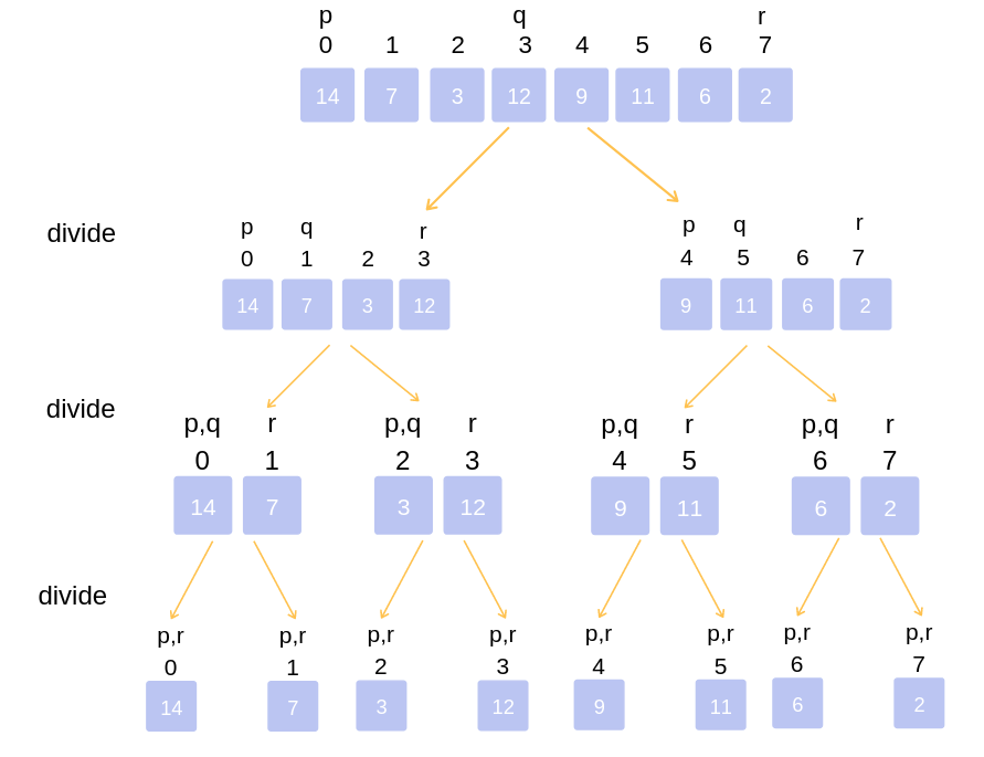
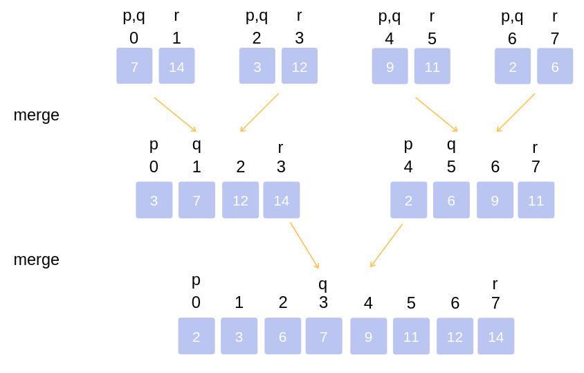
The main idea behind the algorithm is to divide the given array into two parts recursively until it becomes a single element, trivial to sort. The most important part of the algorithm is to merge two sorted arrays into a single array.
Let us first understand how to merge two sorted arrays:
1.We will take two pointers which will point to the starting of the two arrays initially.
2.Then we will take a new, empty auxiliary array with length equal to the sum of lengths of the two sorted arrays.
3.Now, we will compare the elements pointed by our two pointers. And insert the smaller element into the new array and increment that pointer (Assuming we are sorting in non-decreasing order).
4.We continue this process till any of the pointers reach the end of the respective array. Then we insert the remaining elements of the other array in the new array one by one.
(Have a look at the merge function in the following implementation of merge sort)
Now let's understand the merge sort algorithm:
>First of all, we call the mergesort function on the first half and second half of the array.
>Now the two halves are sorted, the only thing to do is to merge them. So we call the merge function.
>We do this process recursively, with the base case that, when the array consists of just one element, it is already sorted and we can return the function call from there.
It's time for an example:
>Let's take an array, Arr[ ]={14,7,3,12,9,11,6,2}.
>Following figure shows each step of dividing and merging the array.
>In the figure, segment (p to q) is the first part and segment (q+1 to r) is the second part of the array at each step.
                                                            // First subarray is arr[l..m]
// Second subarray is arr[m+1..r]
void merge(int Arr[ ], int l, int m, int r)
{
    int n1 = m - l + 1;
    int n2 = r - m;
    // Create temp arrays, for convenience
    int L[n1], R[n2];
    // Copy data to temp arrays L[] and R[]
    for (int i = 0; i < n1; i++)
   	 L[i] = arr[l + i];
    for (int j = 0; j < n2; j++)
   	 R[j] = arr[m + 1 + j];

    // Merge the temp arrays back into arr[l..r]

    // Initial index of the subarrays
    int i = 0, j=0;
    // Initial index of merged subarray
    int k = l;
    while (i < n1 && j < n2) {
   	 if (L[i] <= R[j]) {
   	         arr[k] = L[i];
   	          i++;
   	 }
   	 else {
   	       arr[k] = R[j];
   	        j++;
   	 }
   	 k++;
    }
    while (i < n1) {      // Copy the remaining elements of L[ ], if there are any
   	 arr[k] = L[i];
   	 i++;
   	 k++;
    }
    while (j < n2) {      // Copy the remaining elements of R[ ], if there are any
   	 arr[k] = R[j];
   	 j++;
   	 k++;
    }
}
// l is for left index and r is  right index of the sub-array of arr to be sorted
void mergeSort(int Arr[],int l,int r){
    if(l>=r){
   	 return;    //returns recursively
    }
    int m = (l+r-1)/2;
    mergeSort(Arr,l,m);
    mergeSort(Arr,m+1,r);
    merge(Arr,l,m,r);
}
Time Complexity: The list of size is divided into a max of (log N) parts, and the merging of all sublists into a single list takes O(N) time,hence the worst case run time of this algorithm is O(N logN).
Note:
It is not an in-place sorting algorithm.
Study Material for Merge Sort
STL-sort()
Competitive programmers love C++, STL is one of the reasons. STL i.e. Standard Template Library provides us many in-built useful functions, sort() is one of them. In other words, sort() is one of the most useful STL functions.
Basically, sort() sorts the elements in a range, with time complexity O(N log2N) where N is the length of that range.
It generally takes two parameters , the first one being the point of the array/vector from where the sorting needs to begin and the second parameter being the point up to which we want the array/vector to get sorted. The third parameter is optional and can be used when we want to sort according to some custom rule. By default it sorts in non-decreasing order.
                                                            #include <bits/stdc++.h>
using namespace std;

int main()
{
    int arr[] = { 10, 5,18,99, 6, 7 };
    int n = 6; 	// size of array

    /*Here we take two parameters, the beginning of the
    array and the length n upto which we want the array to
    be sorted*/
    sort(arr, arr + n);

    cout << "\nArray after sorting using "
            "default sort is : \n";
    for (int i = 0; i < n; ++i)
        cout << arr[i] << " ";

    return 0;
}
Output:
Array after sorting using default sort is :
5 6 7 10 18 99
In case we want to sort the complete vector, we should pass vector.begin() and vector.end() as parameters. Further, the vector need not be of basic data types. It can be a vector of pairs, vector of vectors or vector of vectors of pairs etc. In those cases, by default it sorts the objects lexicographically. We can sort it in any particular order using a comparator function.
The third parameter of sort() function, called as the comparator, acts as an operator to compare two elements.
If we did not provide it sort() uses “<” as an operator.
This “comparator” function returns a value; convertible to bool, which tells the sort() function whether the passed “first” argument should be placed before the passed “second” argument or not.
                                                            #include <bits/stdc++.h>
using namespace std;
bool compare(int a, int b)
{
    return (a>b);
 // When this returns true, a will come before b in sorted array
}
int main()
{
   vector<int> v={10, 14, 2, 64, 13};
   int n = v.size();
    // sort in descending order
    sort(v.begin(),v.end(), compare);
    cout << "Vector sorted in descending order is : \n";
    for (int i = 0; i < n; i++)
        cout << v[i] << "  ";
    return 0;
}
Output:
Vector sorted in descending order is :
64 14 13 10 2
Study Material for Sorting
Hashing
Hash Function
Hashing is a key-to-address mapping process:
Hashing is a search technique implemented using the Hashing data structure which uses a special function known as Hash function which map’s a given value with a particular key and creates a hash table which is then used for faster access of elements in constant time independent of the number of values to be searched.
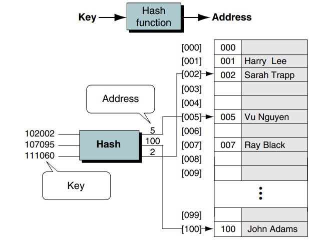
Hash Function:
Hash function is a function that takes a key as an input and converts it to another small practical integer value which is then used as an index in the hash table.
Key -> Hash Function -> Address in hash table
There are various methods to generate/make hash functions, but the trivial and most often used method is, Division Method (Take modulo of given key with another number and use this as index in hash table )
For a good hash function we should consider that it is efficiently computed and the various index positions in the table are equally likely for each key.
Study Material for Hash Function
Hash Table
Similar to the direct access table, it is an array to store pointers/data corresponding to the index location generated for a key by hash function.
Hash table is different from a direct access table for the original range of key as the hash function reduces the range of the original key to a small practical range.
Why to use Hashing ?
In various real life situations we deal with very large values and their associated data for which we need to do insertion,deletion and searching operations.
To search for a given element we have two techniques:
1.Linear Search - Time complexity O(n)
2.Binary Search - Time complexity O(log n)
For storing data, we can use:
1.Array: If we use array and store information then insertion, deletion and searching will have time complexity of O(n).
2.Sorted Array: Searching can be done in O(log n) but we need to sort after each insertion or deletion which increases the time complexity of O(n) to O(n*log n) or more.
3.LinkedList: Insertion, deletion and searching can be done in O(n) time.
4.AVL Tree: Insertion, deletion and searching can be done in O(log2n) time.
5.Direct address table: We can create a list of the size of maximum value we will be dealing with and then use value as index to store data in the array or list, this will make insertion, deletion and searching in O(1) constant time. But it will cost us in terms of memory as to store x data pointers with highest value h (1<= h <= 1050) ,space complexity is of order O(x*h), which is not a feasible solution.
So from the above discussion it can be noticed for such cases, best case for searching is O(log n) and worst case is O(n).
We use Hashing to get the best and average case to be done in O(1) and in the worst case O(n).
Performance of Hash Function:
The performance of hashing can be evaluated under the assumption that each key is equally likely to be hashed to any slot of the table.
n = Number of keys to be inserted in the hash table
m = Number of slots in the hash table
Load factor α = n/m
Study Material for Hash Table
Collision In Hashing
Collision in Hashing:
Using a hash function we get a smaller number for a big key, so there might be a possibility that after processing different keys through a hash function we get the same value. This situation where a newly inserted key maps to an already occupied slot in the hash table is called collision.
Hash(key1) = value
Hash(key2) = value
To handle such situations we use some collision handling technique.
We can use following collision handling technique:
Linear probing
Quadratic probing
Chaining
Double hashing
1. Linear Probing:
We have a hash table of size, more than the number of values to be stored.
In linear probing if there is something stored already at the index v in the hash table, we then check for the (v + 1)%Table_Size th index and so on (increment index by 1) till we find an empty slot in the hash table.
For example, You have a hash function x % 8 and you need to insert values 80,86,88,93,91,102,105,121:
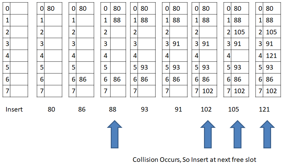
2. Quadratic Probing:
We have a hash table of size L, more than the number of values to be stored.
In quadratic probing if there is something stored already at the index v in the hash table, we then check for the (v + 1*1) %Table_Size index and so on till we find an empty slot in the hash table.
Pattern for finding empty slot:
(v + 1*1) %Table_Size → (v + 2*2) %Table_Size → …... → (v + i*i) %Table_Size
Performance of Linear and Quadratic Probing:
Load factor α = n/m ( < 1 )
Search, Insert and Delete take (1/(1 - α)) time
Problems faced during Linear and Quadratic Probing:
Can be used only when the number of frequencies and keys are known.
A slot can be used even if an input key doesn’t map to it using the hash function.
After some collision resolution it starts taking time to find a free slot or to search an element.
3. Chaining:
In the chaining method of Collision resolution we make each cell of the hash table point to a linked list of records that have the same hash function value. Chaining is simple, but requires additional memory outside the table.
Some points to remember:
This way the Hash table never fills up and we can remove the factor that we need to know the number of keys and frequencies as we have to know in linear and quadratic probing.
As some space in hash table are never used, there is wastage of space.
If the chain becomes long then search time can become O(n) in the worst case.
C++ program to use chaining as Collision resolution method
Performance of Chaining:
If, Load factor α = n/m
Expected time to search = O(1 + α)
Expected time to delete = O(1 + α)
Time complexity of search insert and delete is O(1) if α is O(1)
For example, You have a hash function x % 8 and you need to insert values 80,86,88,93,91,102,105,121:
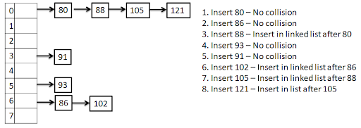
4. Double Hashing:
Double hashing is another collision handling technique in which we apply another hash function to key when a collision occurs.
Let, hash1() and hash2() are the hashing functions.
If using first hashing function there is a collision, we do double hashing using (hash1(key) + i * hash2(key)) % Table_Size, we increment the value of i, till collision is resolved.
Choose such a hash2() function which never evaluates value to zero and also probe all maximum possible indexes in the hash table.
Study Material for Hashing
LEVEL-3: ABLE
Data Structures
Linked List
A linked list is a data structure in which the objects are arranged in a linear order. Unlike an array, though, in which the linear order is determined by the array indices, the order in a linked list is determined by a pointer in each object. Linked lists provide a simple, flexible representation for dynamic sets.
Linked list data set :
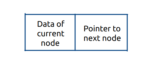
General Linked list :

Singly Linked List
Singly-linked lists contain nodes which have a data field as well as 'next' field, which points to the next node in line of nodes. Operations that can be performed on singly-linked lists include insertion, deletion and traversal.
A singly linked list whose nodes contain two fields: an integer value and a link to the next node
The following code demonstrates how to add a new node with data "value" to the end of a singly linked list:
                                                        node addNode(node head, int value) {
    node temp, p;  // declare two nodes temp and p
    temp = createNode(); // assume createNode creates a new node with data = 0 and next
			       //  pointing to NULL
    temp->data = value;   // add element's value to data part of node
    if (head == NULL)
   {
        head = temp;     // when linked list is empty
    }
    else {
        p = head; // assign head to p
        while (p->next != NULL) {
            p = p->next; // traverse the list until p is the last node. The last node always points
			// to NULL
        }
        p->next = temp; // Point the previous last node to the new node created.
    }
    return head;
}
Study Material for Linked List
Count Pairs whose sum is equal to X
Is linked List Length Even or Odd?
Occurrence of an integer in a Linked List
Delete Alternate Nodes
Stack & Queue (with STL)
Stacks and Queues are dynamic sets in which the element can be added or removed by some predefined operations.
In a stack, it implements LAST IN, FIRST OUT (LIFO). It means whichever element is added at the last will be the one to be removed first.
In a queue, it implements FIRST IN, FIRST OUT (FIFO). It means whichever element is added first will be removed first.
There are several ways to implement stacks and queues on a computer.
Stacks
The insert operation on a stack is often called PUSH, and the delete operation is called POP. These names are allusions to physical stacks, such as the spring-loaded stacks of plates used in cafeterias. The order in which plates are popped from the stack is the reverse of the order in which they were pushed onto the stack since only the top plate is accessible. Below is a visual of how stack data structures work, by inserting and removing elements, which expresses the LIFO property. Let’s define a stack named S.
Stack Definition in c++ : stack < <data type> > <stack name>;
Here we are defining stack if Integer Data Type :
stack< int > S
Push Operations :
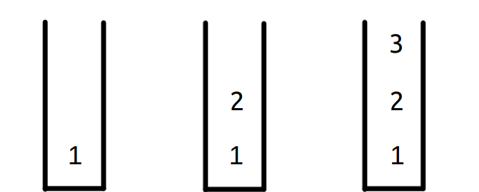
Pop Operations :
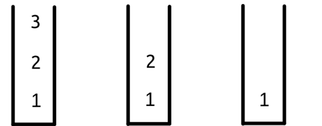
Other Basic operations of Stack :
1 . empty() : checks if the stack is empty.
2. size() : returns the count of elements present in the stack.
3. top() : return the topmost element present in the stack.
When the stack contains no elements, it is said to be empty. The stack can be tested for emptiness by the query operation empty(). If an empty stack is popped, we call it
stack underflows, which is normally an error. And if the count of elements exceeds the maximum limit, we call it stack overflow. We do not worry about stack overflow in the code implementations shown below.
Code Implementations with various operations :
                                                            #include<bits/stdc++.h>
using namespace std;

int main()
{

    stack<int> s; // stack definition

    s.push(1);
    s.push(2);
    s.push(3);

    cout << "The stack size is : " << s.size() << endl; // printing the current
                                                        		         // size of the  stack.

    cout << "The current topmost element : " << s.top() << endl;

    s.pop(); // removing the topmost element.
    cout << "The new current topmost element : " << s.top() << endl;
    cout << "The new size of the stack is : " << s.size() << endl;


    // checking for emptiness of the stack.
    if(s.empty()==true)
        cout << "The stack is empty now.\n";
    else
        cout << "The stack is not empty yet.\n";

    // printing all the elements left in the stack from top to bottom
    cout << "The elements in the stack are : ";
    while( s.empty() == false)
    {
        cout << s.top() << " ";    // printing the topmost element.
        s.pop(); // removing the topmost element so as to access the other elements
                      // in the stack.
    }

    // checking for emptiness of the stack.
    if(s.empty()==true)
        cout << "\nThe stack is empty now.";
    else
        cout << "\nThe stack is not empty yet.";

    return 0;
}
Output :
The stack size is : 3
The current topmost element : 3
The new current topmost element : 2
The new size of the stack is : 2
The stack is not empty yet.
The elements in the stack are : 2 1
The stack is empty now.
Queues
We call the insert operation on a queue as enque, and we call the delete operation dequeue(It is the same as pop in the stack) . The FIFO property of a queue causes it to operate as a line of people in the registrar's office. The queue has a head and a tail. When an element is enqueued, it takes its place at the tail of the queue, just as a newly arriving student takes a place at the end of the line. The element dequeued is always the one at the head of the queue, like the student at the head of the line who has waited the longest.
Below is a visual of how queue data structure works, by inserting and removing elements, which expresses the FIFO property. Let’s define a queue named q.
Queue definition : queue < <data type> > <queue name>;
Here we are defining queue of Integer Data Type :
queue< int > q
Push and Pop Operation :
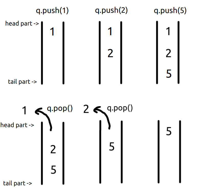
Other Basic Operations in Queue :
1. size() : returns the number of elements in the queue.
2. empty() : checks if the queue is empty.
3. front() : returns the element in front of the queue
4. back() : returns the element at the back of the queue.
Code implementation with various operations :
                                                            int main()
{

      queue<int> q;// defining queue.

      q.push(1);
      q.push(2);
      q.push(5);

      cout << "The queue size is : " << q.size() << endl;

      cout << "The element in front of the queue : " << q.front() << endl;
      cout << "The element at the back of the queue : " << q.back() << endl;

      q.pop();   // removing the element at the front ( Dequeue ).

      cout << "The new element in front of the queue : " << q.front() << endl;
      cout << "The new size of the queue is : " << q.size() << endl;

      if( q.empty() == true )
            cout << "The queue is empty!\n";
      else
            cout << "The queue is not empty yet!\n";

      cout << "The elements in the queue are: ";

      // printing all the elements in the queue from front to back.
      while( q.empty() == false )
      {
            cout << q.front() << " ";
            q.pop();
      }

      if( q.empty() == true )
            cout << "\nThe queue is now empty!";
      else
            cout << "\nThe queue is not empty yet!";

      return 0;
}
Output :
The queue size is : 3
The element in front of the queue: 1
The element at the back of the queue: 5
The new element in front of the queue: 2
The new size of the queue is: 2
The queue is not empty yet!
The elements in the queue are: 2 5
The queue is now empty!
Study Material for Stack & Queue (with STL)
Implement stack using array
Remove repeated digits in a given number
Print Bracket Number
Max sum in sub-arrays
Binary Tree & BST
A binary tree is a special type of tree in which a node can have at most two children.

Binary Tree Representation
Each node contains three components :
1. Pointer to left child
2. Pointer to right child
3. Data element
Code :-
                                                        struct node {
   int data;
   struct node *left;
struct node *right;
};
Types of Binary Trees
1.Full Binary Tree : A full binary tree is A binary tree in which all the nodes have either zero or two children.
2. Complete Binary tree : A complete binary tree is a binary tree in which every level, except possibly the last, is completely filled, and all nodes are as far left as possible.
3.Perfect Binary tree : A perfect binary tree is a binary tree in which every internal node has exactly two child nodes and all the leaf nodes are at the same level
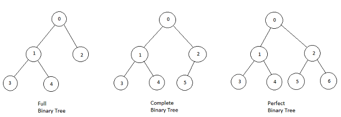
Binary tree traversals:-
A binary Tree can be traversed in two ways:
1. Breadth First Traversal (Or Level Order Traversal)
2. Depth First Traversals
A.Inorder Traversal (Left-Root-Right)
B.Preorder Traversal (Root-Left-Right)
C.Postorder Traversal (Left-Right-Root)
Breadth First Traversal
In BFS, For each node, first the node is visited and then it’s child nodes are put in a queue.This process is repeated till the queue becomes empty.
Code :
                                                        void LevelOrder(Node *root)
{
    // Base Case
    if (root == NULL)  return;

    // Create an empty queue for level order traversal
    queue<Node *> q;

    // Enqueue Root
    q.push(root);

    while (q.empty() == false)
    {
        // Print front of queue and remove it from queue
        Node *node = q.front();
        cout << node->data << " ";
        q.pop();

        /* Enqueue left child */
        if (node->left != NULL)
            q.push(node->left);

        /*Enqueue right child */
        if (node->right != NULL)
            q.push(node->right);
    }
}
Depth First Traversals
Inorder traversal
1.First, visit all the nodes in the left subtree
2.Then the root node
3.Visit all the nodes in the right subtree
Code:-
                                                        void Inorder(struct Node* node)
{
    if (node == NULL)
        return;

    /* first recur on left child */
    Inorder(node->left);

    /* then print the data of node */
    cout << node->data << " ";

    /* now recur on right child */
    Inorder(node->right);
}
Preorder traversal
1.Visit root node
2.Visit all the nodes in the left subtree
3.Visit all the nodes in the right subtree
Code:-
                                                        void Preorder(struct Node* node)
{
    if (node == NULL)
        return;

    /* first print data of node */
    cout << node->data << " ";

    /* then recur on left subtree */
    Preorder(node->left);

    /* now recur on right subtree */
    Preorder(node->right);
}
Postorder traversal
1.Visit all the nodes in the left subtree
2.Visit all the nodes in the right subtree
3.Visit the root node
Code:-
                                                        void Postorder(struct Node* node)
{
    if (node == NULL)
        return;

    // first recur on left subtree
    Postorder(node->left);

    // then recur on right subtree
    Postorder(node->right);

    // now deal with the node
    cout << node->data << " ";
}
Binary Search Tree(BST)
A binary search tree (BST)is a rooted binary tree whose internal nodes each store a key greater than all the keys in the node's left subtree and less than those in its right subtree.The left and right subtree each must also be a binary search tree.
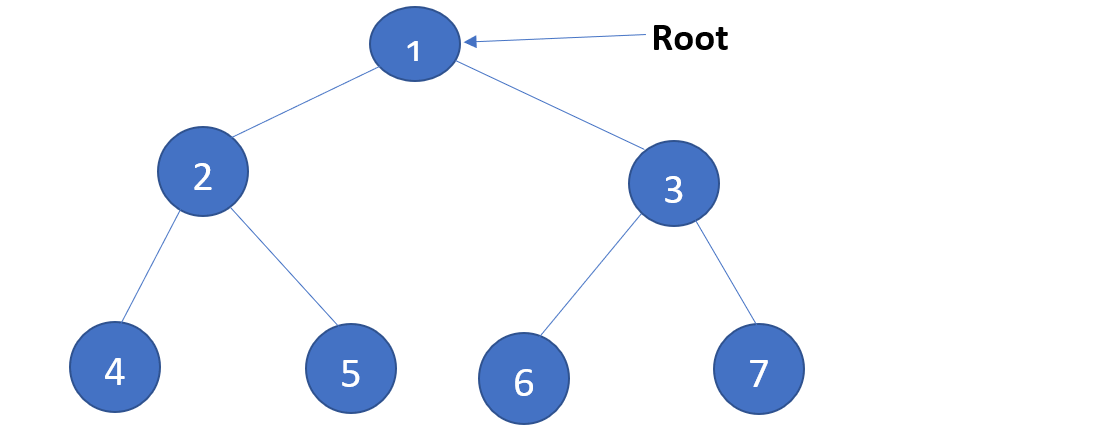
The basic operations of BST are as follows:-
1. Search : For searching an element in the binary search tree.
The algorithm works on the property that in a binary search tree,all the values in the left subtree are less than the particular node and all the values in the right subtree are greater than the particular node.If the value we are searching is less than the root,then the right subtree is not considered and if the value is greater than the root,then the left subtree is not considered.This is done recursively.
Code for the search operation is given below:
                                                        struct node* find(struct node* root, int key)
{
    if (root == NULL ) //If the key is not present in the tree
      return NULL;

    if( root->key == key) // key is present at the root
      return root;

    if (root->key < key) //root's key is less than the key
      return find(root->right, key);

   //root's key is greater than the key
    return find(root->left, key);
}
2. Insert : Inserting an element into the binary search tree.
The new element is inserted in such a way that even after adding the element,the properties of the BST hold true. We Start searching from the root node, if the value to be inserted is less than the data, search for an empty location in the left subtree and insert the data. Otherwise, search for an empty location in the right subtree and insert the data.
Code for insert operation is given below:-
                                                        struct node *insert(struct node *node, int key) {

  // Return a new node if the tree is empty
  if (node == NULL) return newNode(key);

  if (key < node->key)
    node->left = insert(node->left, key);
  else
    node->right = insert(node->right, key);

  return node;
}
3.Delete : Deleting an element present in the BST.
When we have to delete a node in BST,three cases arise:-
i)the node to be deleted is the leaf node
ii)the node to be deleted lies has a single child node
iii)the node to be deleted has two children
Code for the delete operation is given below:-
                                                        struct node *delete(struct node *root, int key) {
  // Return if the tree is empty
  if (root == NULL) return root;

  // Find the node to be deleted
  if (key < root->key)
    root->left = Node(root->left, key);
  else if (key > root->key)
    root->right = Node(root->right, key);
  else {

    // If the node is with only one child or no child
    if (root->left == NULL) {
      struct node *temp = root->right;
      free(root);
      return temp;
    } else if (root->right == NULL) {
      struct node *temp = root->left;
      free(root);
      return temp;
    }

    // If the node has two children
    struct node *temp = minValueNode(root->right);

    // Place the inorder successor in position of the node to be deleted
    root->key = temp->key;

    // Delete the inorder successor
    root->right = deleteNode(root->right, temp->key);
  }
  return root;
}
Study Material for Binary Tree and BST
Heaps and Priority Queue(with STL)
Heap
A Heap is a tree-based data structure in which all the nodes of the tree are in a specific order.
There are two types of Heap :-
1.Max Heap:- In Max Heap, the key of the parent node will always be greater than or equal to the key of the child node across the tree.
2.Min Heap:- In Min Heap, the key of the parent node will always be less than or equal to the key of the child node across the tree.
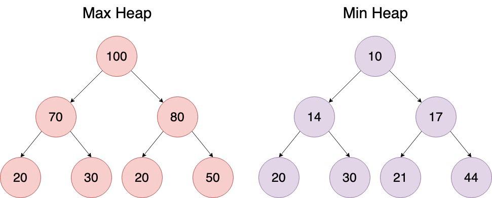
Heap in C++ STL
The heap operations are as follows:-
1.make_heap() : This function converts a range in a container to a heap.
2.front() : This function returns the first element of the heap which is the largest number.
3.push_heap() : This function is used to insert an element into the heap. The size of the heap is increased by 1.
4.pop_heap() : this function is used to delete the largest element of the heap.After deleting an element, the heap elements are reorganized accordingly. The size of heap is decreased by 1.
5.sort_heap() : This function is used to sort the heap in ascending order.
6.is_heap() : This function is used to check whether the container is a heap or not.
7.is_heap_until() : This function returns the iterator to the position till the container is the heap.
Code implementation with various operations :
                                                            #include<bits/stdc++.h>
using namespace std;
int main()
{

    // Initializing a vector
    vector<int> h = {2, 3, 4, 1, 5};

    // Converting vector into a heap using make_heap()
    make_heap(h.begin(), h.end());

    // Displaying the maximum element of heap using front()
    cout<<"The maximum element of heap before push is: "<<h.front()<<endl;

    // using push_back() to enter element  in vector
    h.push_back(6);

    // using push_heap() to reorder elements
    push_heap(h.begin(), h.end());

    cout<<"The maximum element of heap after push is: "<<h.front()<< endl;

    // using pop_heap() to delete maximum element
    pop_heap(h.begin(), h.end());
    h.pop_back();

    cout<< "The maximum element of heap after pop is: "<<h.front()<< endl;

    cout << "The heap elements are : "<<endl;
    for (int &x : h)
       cout << x << " ";
    cout << endl;

    // sorting heap using sort_heap()
    sort_heap(h.begin(), h.end());


    cout << "The heap elements after sorting are : ";
    for (int &x : h)
       cout << x << " ";
}
Output:-
The maximum element of heap is : 5
The maximum element of heap before is : 5
The maximum element of heap after push is : 6
The maximum element of heap after pop is : 5
The heap elements are : 5 4 3 2 1
The heap elements after sorting are : 1 2 3 4 5
Priority queue
A priority queue is an extension of a queue in which each element has a priority associated with it and is served according to its priority. If elements with the same priority occur, they are served according to their order in the queue.
Priority Queue in C++ STL
Syntax for creating priority queue.
priority_queue<int> pq;
Default C++ creates a max heap for priority queue.
The heap operations are as follows :-
1.push() : This function inserts an element in the priority_queue.Its time complexity is O(logN) where N is the size of the priority queue.
2.pop() : This function removes the topmost element from the priority queue, i.e, greatest element.Its time complexity is O(logN) where N is the size of the priority queue.
3.top() : This function returns the element at the top of the priority queue which is the greatest element present in the queue.Its time complexity is O(1).
4.size() : this function returns the size of the priority queue.Its time complexity is O(1).
5.empty() : this function returns boolean true if the priority queue is empty and false, if it’s not empty.Its time complexity is O(1).
6.swap() : This function is used to swap the contents of one priority queue with another priority queue of the same type and size.
Code implementation with various operations :
                                                            #include <bits/stdc++.h>
using namespace std;

int main()
{
    priority_queue<int> pq;
    pq.push(1);
    pq.push(3);
    pq.push(2);
    pq.push(5);
    pq.push(4);

    cout << "The priority queue pq is : "<<endl;
        while(!pq.empty())
        {
        std::cout << pq.top() << ' ';
        pq.pop();
        }


    pq.push(1);
    pq.push(3);
    pq.push(2);
    pq.push(5);
    pq.push(4);

    cout << "The size of the priority queue is : " << pq.size()<<endl;
    cout << "The largest element is the priority queue is  : "<< pq.top()<<endl;

    //removing the largest element
    pq.pop();

     cout << "The priority queue pq after pop() operation is  : ";
        while(!pq.empty())
        {
        std::cout << pq.top() << ' ';
        pq.pop();
        }
}
Output:-
The priority queue pq is : 5 4 3 2 1
The size of the priority queue is : 5
The largest element is the priority queue is : 5
The priority queue pq after pop() operation is : 4 3 2 1
Study Material for Heap and Priority Queue(with STL)
STL
Iterator
The C++ STL (Standard Template Library) is a powerful set of C++ template classes to provide general-purpose classes and functions with templates that implement many popular and commonly used algorithms and data structures like vectors, lists, queues, and stacks.
C++ Standard Template Library is made up of following three well-structured components −
Containers : Containers are used to manage collections of objects of a certain kind. There are several different types of containers like deque, list, vector, map etc.
Algorithms : Algorithms are defined as collections of functions especially designed to be used on ranges of elements.They act mainly on containers and provide means for various operations for the contents of containers.
Iterators : Iterators are used for working upon a sequence of different elements.These sequences may be containers.They are major features that allow generality in STL.
Iterator:
An iterator is any object that, points to some element in a range of elements (such as an array or a container) and has the ability to iterate through those elements using a set of operators (with at least the increment (++) and dereference (*) operators).
A pointer is a form of an iterator. A pointer can point to elements in an array, and can iterate over them using the increment operator (++). There can be other types of iterators as well. For each container class, we can define an iterator which can be used to iterate through all the elements of that container.
Example:
vector<int>::iterator it; // creates iterator it for vector container
Implementation:
                                                            #include <iostream>
#include <vector>   //for vector container
#include <iterator> //for iterator
using namespace std;

int main()
{
    vector<int> v={1,2,3,4,5};

    //declaration of iterator to vector
    vector<int>::iterator it;

    //displaying elements in the vector using iterator
    for(it=v.begin();it!=v.end();it++)
    {
        cout<<*it<<" ";
    }
    cout<<"\n";
    return 0;
}
Output:
1 2 3 4 5
Pair
Pair:
Pair is a container that can be used to bind together two values which may be of different types. Pair provides a way to store two heterogeneous objects as a single unit.
One must include a <utility> header file to use the pair.
Different ways to declare and initialize pair are:
                                                        pair < char , int > p1;         //creates a default pair
pair < char , int >p2 (‘a’,1);      //initialisation of pair p2
pair < char , int > p3(p2);      //creates a copy of p2
                                                            p1 = make_pair(2, ‘b’);

pair_name.first;      //gives access to the first element
pair_name.second;   //gives access to the second element
We can also initialize a pair using make_pair() function.It will return a pair with the first element set to x and second element set to y.
To access the elements we use keywords, first and second to access the first and second element respectively.
Implementation:
                                                            #include <bits/stdc++.h>
using namespace std;

int main()
{
    pair <int, char> p;     //declaration of pair
    pair <int, char> p1(2, 'b');
    p = make_pair(1, 'a');
    cout << p.first << ' ' <<  p.second << endl;
    cout << p1.first << ' ' << p1.second << endl;
    return 0;
}
Output:
1 a
2 b
String
String:
C++ provides a powerful alternative for the char*. It is not a built-in data type, but is a container class in the Standard Template Library. String class provides different string manipulation functions like concatenation, find, replace etc.
<string> is a header file that contains functions of string containers.
Different ways to declare strings are:
string s ;
Creates empty string s
string s1(“Hello World”);
Creates string s1 storing Hello World
string s1(s2) ;
Creates a copy s1 of another string s2
string s1( s2,1,3);
Creates a string s1 storing substring of s2 from index 1 to index 3
string s1(“Hello World”,5);
Creates a string s1 storing “Hello” that is only 5 characters of passed string
string s1(5,”*”);
Creates string s1 storing “*****”
string s2(s1.begin(),s1.end());
Creates a copy of s1 using iterators.
Some of the member functions of string:
•append(): Inserts additional characters at the end of the string (can also be done using ‘+’ or ‘+=’ operator). Its time complexity is O(N) where N is the size of the new string.
Syntax to add str2 at the end of str1:
str1.append(str2)
•assign(): Assigns new string by replacing the previous value (can also be done using ‘=’ operator).
Syntax to assign str2 to str1:
str1.assign(str2)
•at(): Returns the character at a particular position (can also be done using ‘[ ]’ operator). Its time complexity is O(1).
Syntax to print character at index idx of string str:
str.at(idx)
•begin(): Returns an iterator pointing to the first character. Its time complexity is O(1).
Syntax:
string_name.begin()
•clear(): Erases all the contents of the string and assign an empty string (“”) of length zero. Its time complexity is O(1).
Syntax:
string_name.clear()
•compare(): Compares the value of the string with the string passed in the parameter and returns an integer accordingly. If both the strings are equal then it returns 0,if string s2 is greater than that of s1 then it returns value greater than zero otherwise it returns value less than zero.Its time complexity is O(N + M) where N is the size of the first string and M is the size of the second string.
Syntax to compare two strings:
s1.compare(s2)
Syntax to compare string s1 with s2 from idx index of s2 for len characters:
s2.compare(idx,len,s1)
•copy(): Copies the substring of the string in the string passed as parameter and returns the number of characters copied. Its time complexity is O(N) where N is the size of the copied string.
Syntax to copy s2 to s1:
s1.copy(s2)
•c_str(): Convert the string into a C-style string (null terminated string) and return the pointer to the C-style string. Its time complexity is O(1).
•empty(): Returns a boolean value, true if the string is empty and false if the string is not empty. Its time complexity is O(1).
Syntax:
string_name.empty()
•end(): Returns an iterator pointing to a position which is next to the last character. Its time complexity is O(1).
Syntax:
string_name.end()
•erase(): Deletes a substring of the string. Its time complexity is O(N) where N is the size of the new string.
Syntax to delete a character at position pos from string:
string_name.erase(pos)
Syntax to delete characters from a given range [pos1,pos2):
string_name.erase(pos1,pos2)
Syntax to remove substring of length len from index idx:
string_name.erase(idx,len)
•find(): Searches the string and returns the first occurrence of the parameter in the string. Its time complexity is O(N) where N is the size of the string.
Syntax to find str2 from str1:
str1.find(str2)
•insert(): Inserts additional characters into the string at a particular position. Its time complexity is O(N) where N is the size of the new string.
•length(): Returns the length of the string. Its time complexity is O(1).
Syntax:
string_name.length()
•replace(): Replaces the particular portion of the string. Its time complexity is O(N) where N is the size of the new string.
Syntax to replace len characters from pos position of str1 with str2:
str1(pos,len,str2)
•resize(): Resize the string to the new length which can be less than or greater than the current length.If new size is greater than that of original one then character passed as parameter is added to string to make it of new size. Its time complexity is O(N) where N is the size of the new string.
Syntax :
string_name.resize(new_size,character)
•size(): Returns the length of the string. Its time complexity is O(1).
Syntax:
string_name.size()
•substr(): Returns a string which is the copy of the substring of range [pos,pos+len) where pos is position and len is length given as parameters.Its time complexity is O(N) where N is the size of the substring.
Syntax:
string_name.substr(pos,len)
Implementation:
                                                            #include <bits/stdc++.h>
using namespace std;

int main()
{
    string s, s1;
    s = "HELLO";
    s1 = "HELLO";

    //compares the two strings s and s1
    if(s.compare(s1) == 0)
        cout << s << " is equal to " << s1 << endl;
    else
        cout << s << " is not equal to " << s1 << endl;

    //append to s
    s.append(" WORLD!");
    cout << s << endl;
    cout<<s.c_str()<<"\n";

    //compares the two string s and s1
    if(s.compare(s1) == 0)
        cout << s << " is equal to " << s1 << endl;
    else
        cout << s << " is not equal to " << s1 << endl;
    return 0;
}
Output:
HELLO is equal to HELLO
HELLO WORLD!
HELLO WORLD!
HELLO WORLD! is not equal to HELLO
Vector
Same as dynamic arrays,vectors are STL containers having the ability to resize itself automatically when an element is inserted or deleted, with their storage being handled automatically by the container. Vector elements are placed in contiguous storage so that its elements can be accessed and traversed using iterators just as efficiently as in arrays.
One must include a <vector> header file to use vectors.
Ways to create vectors:
vector<data_type> v;
Creates an empty vector v without any element.
vector<data_type> v1(v2) ;
Creates a copy of another vector of the same type.(all elements of v2 is copied to v1)
vector<data_type> v(n);
Creates a vector v with n elements that are created by the default constructor.
vector<data_type> v(n,element);
Creates a vector v initialised with n copies of element elem.
vector<data_type> v(beg,end);
Creates a vector v initialised with the elements of range [beg,end).
Some of the member functions of vectors are:
•at():It returns a reference to the element at specified position in the vector.Its time complexity is O(1).
Syntax:
vector_name.at(val)
where val is the position to be fetched.
•insert():Inserts new elements into the vector at a particular position. Its time complexity is O(N + M) where N is the number of elements inserted and M is the number of the elements moved .
Syntax to insert element val at position pos:
vector_name.insert(pos,val)
•push_back():Inserts a new element at the end of the vector. Its time complexity is O(1).
Syntax:
vector_name.push_back(val)
where val is the element to be inserted.
•pop_back():Removes the last element from the vector. Its time complexity is O(1).
Syntax:
vector_name.pop_back()
•begin():It is a function which returns an iterator pointing to the first element of the vector.Its time complexity is O(1).
Syntax:
vector_name.begin()
•end():It is a function which returns an iterator pointing to next to the last element of the vector.Its time complexity is O(1).
Syntax:
vector_name.end()
•back():It returns a reference to the last element in the vector.Its time complexity is O(1).
Syntax:
vector_name.back()
•front():It returns a reference to the element at specified position in the vector.Its time complexity is O(1).
Syntax:
vector_name.front()
•clear():Deletes all the elements from the vector and assigns an empty vector. Its time complexity is O(N) where N is the size of the vector.
Syntax:
vector_name.clear()
•size():It is a function which returns the number of elements present in the vector.Its time complexity is O(1).
Syntax:
vector_name.size()
•empty():It is a function which is used to check whether the vector is empty or not.It returns true if the vector is empty otherwise returns false.Its time complexity is O(1).
Syntax:
vector_name.empty()
•erase():It is a function used to remove elements from the specified position of the vector.
Its time complexity is O(N + M) where N is the number of the elements erased and M is the number of the elements moved.
Syntax to remove element at a specified position pos:
vector_name.erase(pos);
Syntax to remove elements from a given range [pos1,pos2):
vector_name.erase(pos1,pos2)
•resize():This function resizes the container so that its size becomes n.This function alters the container by removing or inserting values in the vector.Its time complexity is O(N) where N is the size of the resized vector.
Syntax:
vector_name.resize(n,val)
where n is the new container size and val is the value to be inserted if the new size exceeds current one.
Implementation:
                                                            #include <bits/stdc++.h>
using namespace std;

int main() {

    vector<int> v;

    //insert 5 values in vector v
    for(int i=1;i<=5;i++)
    {
        v.push_back(i);
    }

    //to print the values of vector
    for(auto it=v.begin();it!=v.end();it++)
    {
        cout<<" "<<*it;
    }
    cout<<"\n";

    cout<<"size of the vector:"<<v.size()<<"\n";
    cout<<"value of at 3rd index:"<<v.at(3)<<"\n";     //finding value store at index 3

    //Inserting three 6 at the end of the vector
    v.insert(v.end(),3,6);
    //to print the values of vector
    for(auto it=v.begin();it!=v.end();it++)
    {
        cout<<" "<<*it;
    }
    cout<<"\n";

    //removes last element
    v.pop_back();
    v.pop_back();

    //to print the values of vector
    for(auto it=v.begin();it!=v.end();it++)
    {
        cout<<" "<<*it;
    }
    cout<<"\n";

    v.insert(v.begin(),3,7);   //inserts three 7 at the beginning
    //to print the values of vector
    for(auto it=v.begin();it!=v.end();it++)
    {
        cout<<" "<<*it;
    }
    cout<<"\n";

    //sort the vector v in increasing order
    sort(v.begin(),v.end());

    //to print the values of vector
    for(auto it=v.begin();it!=v.end();it++)
    {
        cout<<" "<<*it;
    }
    cout<<"\n";

    if(v.empty())
       cout<<"vector is empty"<<"\n";
    else
       cout<<"vector is not empty"<<"\n";

    v.resize(v.size()+6,4);
    //to print the values of vector
    for(auto it=v.begin();it!=v.end();it++)
    {
        cout<<" "<<*it;
    }
    cout<<"\n";

    cout<<"Size before using clear function:"<<v.size()<<"\n";
    v.clear();
    cout<<"Size after using clear function:"<<v.size()<<"\n";

    // your code goes here
    return 0;
}
Output:
1 2 3 4 5
size of the vector:5
value of at 3rd index:4
1 2 3 4 5 6 6 6
1 2 3 4 5 6
7 7 7 1 2 3 4 5 6
1 2 3 4 5 6 7 7 7
vector is not empty
1 2 3 4 5 6 7 7 7 4 4 4 4 4 4
Size before using clear function:15
Size after using clear function:0
List
Lists are sequence containers that allow non-contiguous memory allocation. As compared to vector, list has slow traversal, but once a position has been found, insertion and deletion are quick.It is implemented as Doubly linked list in STL.
One must include a <list> header file to use list.
Syntax to declare list:
list<data_type> list_name
Some of the member function of List:
•begin():It is a function which returns an iterator pointing to next to the last element of the list.Its time complexity is O(1).
Syntax:
list_name.end()
•end():It is a function which returns an iterator pointing to next to the last element of the list.Its time complexity is O(1).
Syntax:
list_name.end()
•push_back():It adds a new element at the end of the list, after its current last element. Its time complexity is O(1).
Syntax to insert val at the end of the list:
list_name.push_back(val)
•pop_back():It removes the last element of the list, thus reducing its size by 1. Its time complexity is O(1).
Syntax to remove the last element of the list
list_name.pop_back()
•push_front():It adds a new element at the front of the list, before its current first element. Its time complexity is O(1).
Syntax to insert val at the beginning of the list:
list_name.push_front(val)
•pop_front():It removes the first element of the list, thus reducing its size by 1. Its time complexity is O(1).
Syntax to remove first element of the list:
list_name.pop_front()
•front():It returns a reference to the element at specified position in the list.Its time complexity is O(1).
Syntax:
list_name.front()
•back():It returns a reference to the last element in the list.Its time complexity is O(1).
Syntax:
list_name.back()
•assign(): It assigns new elements to the list by replacing its current elements and changing its size accordingly.It time complexity is O(N).
Syntax to replace n number of elements from beginning with val
list_name.assign(n,val)
•insert():It inserts new elements in the list before the element on the specified position. Its time complexity is O(N).
Syntax for inserting n elements having value val before pos
list_name.insert(pos,n,val)
•erase():It removes all the elements from the list, which are equal to the given element. Its time complexity is O(N).
Syntax to remove element from a specified position:
list_name.erase(pos)
Syntax to remove element from given range [pos1,pos2):
list_name.erase(pos1,pos2)
•remove():It removes all the elements from the list, which are equal to the given element passed as parameter. Its time complexity is O(N).
Syntax:
list_name.remove(val)
•empty():It is a function which is used to check whether the list is empty or not.It returns 1 if the list is empty otherwise it returns 0.Its time complexity is O(1).
Syntax:
list_name.empty()
•size():It returns the number of elements in the list. Its time complexity is O(1).
Syntax :
list_name.size()
•reverse():It reverses the order of elements in the list. Its time complexity is O(N).
Syntax:
list_name.reverse()
Implementation:
                                                            #include<bits/stdc++.h>
using namespace std;

int main()
{
    list<int> l; //creating list l of int type

    //adding values to the end of the list
    for(int i=1;i<=5;i++)
    {
        l.push_back(i);
    }

    //printing values stored in list
    for(auto it=l.begin();it!=l.end();it++)
    {
        cout<<*it<<" ";
    }
    cout<<"\n";

    //to add value at the front of the list
    l.push_front(7);
    l.push_front(6);

    //printing values stored in list
    for(auto it=l.begin();it!=l.end();it++)
    {
        cout<<*it<<" ";
    }
    cout<<"\n";

   auto f=l.front();
   auto b=l.back();

   cout<<"front element of the list:"<<f<<"\n";
   cout<<"last element of the list:"<<b<<"\n";

    //removing a value from list
      l.remove(6);

    for(auto it=l.begin();it!=l.end();it++)
    {
        cout<<*it<<" ";
    }
    cout<<"\n";

    cout<<"list after reversing the values:\n";
    l.reverse();
    //printing values stored in list
    for(auto it=l.begin();it!=l.end();it++)
    {
        cout<<*it<<" ";
    }
    cout<<"\n";

    cout<<"size of the list before removing values:"<<l.size()<<"\n";

    auto it1=l.begin();
    it1++;
    it1++;
    it1++;
    it1++;
    auto it2=l.end();
    it2--;
    it2--;
    l.erase(it1,it2);
    //printing values stored in list
    for(auto it=l.begin();it!=l.end();it++)
    {
        cout<<*it<<" ";
    }
    cout<<"\n";

    cout<<"size of the element after using erase function:"<<l.size()<<"\n";

    return 0;
}
Output:
1 2 3 4 5
6 7 1 2 3 4 5
front element of the list:6
last element of the list:5
7 1 2 3 4 5
list after reversing the values:
5 4 3 2 1 7
size of the list before removing values:6
5 4 3 2 1 7
size of the element after using erase function:6
Set
Sets are associative containers which store unique values in sorted order. The value of the element cannot be modified once it is added to the set, though it is possible to remove and add the modified value of that element.
One must include a <set> header file to use set.
Ways to create set are:
set<data_type> set_name
Creates an empty set
set<data_type> s1(arr,arr+n)
Creates set s1 from a given array arr of size n
set<data_type> s2(s1)
Creates a copy s2 of set s1
set<data_type> s2(s1.begin(),s1.end())
Creates a copy s2 of set s1 using iterators
Some of the member functions of set are:
•begin():It is a function which returns an iterator pointing to the first element of the set.Its time complexity is O(1).
Syntax:
set_name.begin()
•end():It is a function which returns an iterator pointing to next to the last element of the set.Its time complexity is O(1).
Syntax:
set_name.end()
•insert():It inserts new elements in the set passed as parameter.Its time complexity is O(logN) where N is the size of the set.
Syntax:
set_name,insert(val)
•count():It returns 1 if the element passed as parameter is present otherwise 0.Its time complexity is O(logN) where N is the size of the set.
Syntax:
set_name.count(val)
•find():It returns the iterator pointing to the position where the value passed as parameter is present.If the value is not present in the set then it returns iterator pointing to s.end()
where s is the name of the set.Its time complexity is O(logN) where N is the size of the set.
Syntax:
set_name.find(val)
•erase():Deletes a particular element or a range of elements from the set. Its time complexity is O(N) where N is the number of elements deleted.
Syntax to remove element at position pos:
set_name.erase(pos)
Syntax to remove elements from a given range [pos1,pos2):
set_name.erase(pos1,pos2)
•empty():Returns true if the set is empty and false if the set has at least one element. Its time complexity is O(1).
Syntax:
set_name.empty()
•clear():Deletes all the elements in the set and the set will be empty. Its time complexity is O(N) where N is the size of the set.
Syntax:
set_name.clear()
•size():It returns the number of elements in the set. Its time complexity is O(1).
Syntax :
set_name.size()
Implementation:
                                                            #include<bits/stdc++.h>
using namespace std;

int main()
{
    set<int> s;

    //to insert values in the set
    s.insert(1);
    s.insert(2);
    s.insert(6);
    s.insert(4);
    s.insert(4);  //won't insert 4 as 4 already present in set s
    s.insert(3);
    s.insert(5);

    //to print all values present in the set
    for(auto it=s.begin();it!=s.end();it++)
    {
        cout<<*it<<" ";
    }
    cout<<"\n";

    cout<<"count of 4 present in set s:"<<s.count(4)<<"\n";

    //checks whether 8 present or not
    if(s.find(8)==s.end())
        cout<<"8 not present"<<"\n";
    else
        cout<<"8 is present in the set\n";

    //to erase 5 from the set
    s.erase(5);

    cout<<"Set after removal of 5 from the set"<<"\n";

    //to print all values present in the set
    for(auto it=s.begin();it!=s.end();it++)
    {
        cout<<*it<<" ";
    }
    cout<<"\n";

    //prints the size of the set
    cout<<"Size of the set:"<<s.size()<<"\n";
    return 0;
}
Output:
1 2 3 4 5 6
count of 4 present in set s:1
8 not present
Set after removal of 5 from the set
1 2 3 4 6
Size of the set:5
Multiset
Multiset is a set container which has all the functions same as that of set but with an exception that it can hold the same value multiple times.
Syntax for creating a multiset:
multiset<data_type> multiset_name
Some of the member functions of set are:
•begin():It is a function which returns an iterator pointing to the first element of the multiset.Its time complexity is O(1).
Syntax:
set_name.begin()
•end():It is a function which returns an iterator pointing to next to the last element of the multiset.Its time complexity is O(1).
Syntax:
set_name.end()
•insert():It inserts new elements in the multiset passed as parameter.Its time complexity is O(log N) where N is the size of the multiset.
Syntax:
set_name.insert(val)
•count():It returns the count of numbers of elements whose values are equal to the value passed as parameter.Its time complexity is O(log N) where N is the size of the multiset.
Syntax:
set_name.count(val)
•find():It returns the iterator pointing to the position where the value passed as parameter is present.If the value is not present in the set then it returns iterator pointing to s.end()
where s is the name of the multiset.Its time complexity is O(log N) where N is the size of the size of the multiset.
Syntax:
set_name.find(val)
•erase():Deletes a particular element or a range of elements from the set. Its time complexity is O(N) where N is the number of elements deleted.
Syntax to remove element at position pos:
set_name.erase(pos)
Syntax to remove elements from a given range [pos1,pos2):
set_name.erase(pos1,pos2)
•empty():Returns true if the set is empty and false if the set has at least one element. Its time complexity is O(1).
Syntax:
set_name.empty()
•clear():Deletes all the elements in the set and the set will be empty. Its time complexity is O(N) where N is the size of the set.
Syntax:
set_name.clear()
•size():It returns the number of elements in the set. Its time complexity is O(1).
Syntax :
set_name.size()
Implementation:
                                                            #include <bits/stdc++.h>
using namespace std;
int main()
{

    multiset<int> s;

    //insert elements
    s.insert(1);
    s.insert(6);
    s.insert(2);
    s.insert(5);
    s.insert(3);
    s.insert(3);
    s.insert(5);
    s.insert(3);    //it allows multiple copies of the same value as in here 3.

    // prints the multiset elements
    cout << "The multiset elements are: ";
    for (auto it = s.begin(); it != s.end(); it++)
        cout << *it << " ";

    //to count number of 3
    cout<<"\n"<<s.count(3)<<"\n";

    auto it1=s.find(6);
    cout<<*it1<<"\n";

    s.erase(s.begin());

    // prints the multiset elements after erasing the elements of the given range
    cout << "\nThe multiset elements are: ";
    for (auto it = s.begin(); it != s.end(); it++)
        cout << *it << " ";

    return 0;
}
Output:
The multiset elements are: 1 2 3 3 3 5 5 6
3
6
The multiset elements are: 2 3 3 3 5 5 6
Unordered set
It is an associative container that contains an unordered set of data inserted randomly. Each element may occur only once, so duplicates are not allowed. A user can create an unordered set by inserting elements in any order and an unordered set will return data in any order i.e. unordered form.The main reasons when unordered set can be used are when no sorted data is required means the data is available in an unordered format,when only unique data is needed,when we want to use hash table instead of a binary search tree and when a faster search is required as it take O(1) in average case and O(n) in worst case.
One must include <unordered_set> header file to use unordered_set.
Syntax for creating unordered_set:
unordered_set<int> s; //creates an empty unordered set
unordered_set<int> s={1,2,3,4}; //creates an unordered set containing 1,2,3 and 4
Some of the member functions of set are:
begin():It is a function which returns an iterator pointing to the first element of the unordered set.Its time complexity is O(1).
Syntax:
unordered_set_name.begin()
end():It is a function which returns an iterator pointing to next to the last element of the unordered set.Its time complexity is O(1).
Syntax:
unordered_set_name.end()
insert():It inserts new elements in the unordered set passed as parameter.Its time complexity is O(1) in average case but O(N) in worst case where N is the size of the unordered set.
Syntax:
unordered_set_name,insert(val)
count():It returns 1 if the element passed as parameter is present otherwise 0.Its time complexity is O(1) in average case but O(N) in worst case where N is the size of the unordered set.
Syntax:
unordered_set_name.count(val)
find():It returns the iterator pointing to the position where the value passed as parameter is present.If the value is not present in the unordered set then it returns iterator pointing to s.end() where s is the name of the set.Its time complexity is O(1) in average case but O(N) in worst case where N is the size of the unordered set.
Syntax:
unordered_set_name.find(val)
erase():Deletes a particular element or a range of elements from the unordered set. Its time complexity is O(N) where N is the number of elements deleted.
Syntax to remove element at position pos:
unordered_set_name.erase(pos)
Syntax to remove elements from a given range [pos1,pos2):
unordered_set_name.erase(pos1,pos2)
empty():Returns true if the unordered set is empty and false if the unordered set has at least one element. Its time complexity is O(1).
Syntax:
unordered_set_name.empty()
clear():Deletes all the elements in the unordered set and the unordered set will be empty. Its time complexity is O(N) where N is the size of the unordered set.
Syntax:
unordered_set_name.clear()
size():It returns the number of elements in the unordered set. Its time complexity is O(1).
Syntax :
unordered_set_name.size()
Implementation:
                                                            #include <iostream>
#include <unordered_set>
using namespace std;

int main() {

    unordered_set<int> s;
    unordered_set<int> s1={10,12,11,15};

    //inserting elements in the unordered set
    s.insert(2);
    s.insert(3);
    s.insert(1);
    s.insert(3);
    s.insert(4);
    s.insert(8);
    s.insert(7);
    s.insert(8);

    //printing the elements present in the unordered set
    //like set it will contain unique values but not in order.
    cout<<"Elements present in unordered set s:"<<"\n";
    for(auto it=s.begin();it!=s.end();it++)
    {
        cout<<*it<<" ";
    }
    cout<<"\n";

    //printing the unordered set s1
    cout<<"Elements present in unordered set s1:"<<"\n";
    for(auto it=s1.begin();it!=s1.end();it++)
    {
        cout<<*it<<" ";
    }
    cout<<"\n";

    cout<<"count of 3 in unordered set s:"<<s.count(3)<<"\n";    //gives count of 3 in set s
    cout<<"size of the unordered set s:"<<s.size()<<"\n";        //gives the size of the unordered set s

    //to check the presence of 5 in the unordered set
    if(s.find(5)==s.end())
    {
        cout<<"5 not present in the set s\n";
    }
    else
    {
        cout<<"5 present in the set s\n";
    }

    auto it=s.begin();
    s.erase(it);                         //erase the first element from the unordered set s

    //printing the unordered set
    cout<<"Elements present in unordered set s:"<<"\n";
    for(auto itr=s.begin();itr!=s.end();itr++)
    {
        cout<<*itr<<" ";
    }
    cout<<"\n";

    //swapping the two unordered sets s and s1
    s.swap(s1);

    //printing the unordered set s after swapping
    cout<<"Elements present in unordered set s after swapping:"<<"\n";
    for(auto it=s.begin();it!=s.end();it++)
    {
        cout<<*it<<" ";
    }
    cout<<"\n";

    //printing the unordered set s1 after swapping
    cout<<"Elements present in unordered set s1 after swapping:"<<"\n";
    for(auto it=s1.begin();it!=s1.end();it++)
    {
        cout<<*it<<" ";
    }
    cout<<"\n";

    return 0;
}
Output:
Elements present in unordered set s:
7 3 8 2 1 4
Elements present in unordered set s1:
11 12 15 10
count of 3 in unordered set s:1
size of the unordered set s:6
5 not present in the set s
Elements present in unordered set s:
3 8 2 1 4
Elements present in unordered set s after swapping:
11 12 15 10
Elements present in unordered set s1 after swapping:
3 8 2 1 4
Unordered Multiset
Unordered Multiset:
Unordered multiset is an associative container that contains a set of possibly non-unique objects of type Key. Search, insertion, and removal have average constant-time complexity.
Internally, the elements are not sorted in any particular order, but organized into buckets. Which bucket an element is placed into depends entirely on the hash of its value.This allows fast access to individual elements, since once hash is computed, it refers to the exact bucket the element is placed into.
One must include <unordered_set> header file to use multiset.
Syntax for creating unordered_multiset:
                                                        unordered_multiset<int> s;     //creates an empty unordered multiset
unordered_multiset<int> s={1,2,3,4};   //creates an unordered multiset containing 1,2,3 and 4
Some of the member functions of set are:
begin():It is a function which returns an iterator pointing to the first element of the unordered multiset.Its time complexity is O(1).
Syntax:
unordered_multiset_name.begin()
end():It is a function which returns an iterator pointing to next to the last element of the unordered multiset.Its time complexity is O(1).
Syntax:
unordered_multiset_name.end()
insert():It inserts new elements in the unordered multiset passed as parameter.Its time complexity is O(1) in average case but O(N) in worst case where N is the size of the unordered multiset.
Syntax:
unordered_multiset_name,insert(val)
count():It returns the count of the element passed as parameter. Its time complexity is O(N) where N is the number of elements counted.
Syntax:
unordered_multiset_name.count(val)
find():It returns the iterator pointing to the position where the value passed as parameter is present.If the value is not present in the unordered multiset then it returns iterator pointing to s.end() where s is the name of the unordered multiset.Its time complexity is O(1) in average case but O(N) in worst case where N is the size of the unordered multiset.
Syntax:
unordered_multiset_name.find(val)
erase():Deletes a particular element or a range of elements from the unordered multiset. Its time complexity is O(N) where N is the number of elements deleted.
Syntax to remove element at position pos:
unordered_multiset_name.erase(pos)
Syntax to remove elements from a given range [pos1,pos2):
unordered_multiset_name.erase(pos1,pos2)
empty():Returns true if the unordered multiset is empty and false if the unordered multiset has at least one element. Its time complexity is O(1).
Syntax:
unordered_multiset_name.empty()
clear():Deletes all the elements in the unordered multiset and the unordered multiset will be empty. Its time complexity is O(N) where N is the size of the unordered multiset.
Syntax:
unordered_multiset_name.clear()
size():It returns the number of elements in the unordered multiset. Its time complexity is O(1).
Syntax :
unordered_multiset_name.size()
Implementation:
                                                            #include <iostream>
#include <unordered_set>
using namespace std;

int main() {

    unordered_multiset<int> s;
    unordered_multiset<int> s1={10,12,11,15};

    //inserting elements in the unordered multiset
    s.insert(2);
    s.insert(3);
    s.insert(1);
    s.insert(3);
    s.insert(4);
    s.insert(8);
    s.insert(7);
    s.insert(8);

    //printing the elements present in the unordered multiset
    //like multiset it will contain unique values but not in order.
    cout<<"Elements present in unordered multiset s:"<<"\n";
    for(auto it=s.begin();it!=s.end();it++)
    {
        cout<<*it<<" ";
    }
    cout<<"\n";

    //printing the unordered multiset s1
    cout<<"Elements present in unordered multiset s1:"<<"\n";
    for(auto it=s1.begin();it!=s1.end();it++)
    {
        cout<<*it<<" ";
    }
    cout<<"\n";

     //gives count of 3 in multiset s
    cout<<"count of 3 in unordered multiset s:"<<s.count(3)<<"\n";
            //gives the size of the unordered multiset s
    cout<<"size of the unordered multiset s:"<<s.size()<<"\n";

            //to check the presence of 5 in the unordered multiset
    if(s.find(5)==s.end())
    {
        cout<<"5 not present in the multiset s\n";
    }
    else
    {
        cout<<"5 present in the multiset s\n";
    }

    auto it=s.begin();
    s.erase(it);    //erase the first element from the unordered multiset s

    //printing the unordered multiset
    cout<<"Elements present in unordered multiset s:"<<"\n";
    for(auto itr=s.begin();itr!=s.end();itr++)
    {
        cout<<*itr<<" ";
    }
    cout<<"\n";

    //swapping the two unordered multisets s and s1
    s.swap(s1);

    //printing the unordered multiset s after swapping
    cout<<"Elements present in unordered multiset s after swapping:"<<"\n";
    for(auto it=s.begin();it!=s.end();it++)
    {
        cout<<*it<<" ";
    }
    cout<<"\n";

    //printing the unordered multiset s1 after swapping
    cout<<"Elements present in unordered multiset s1 after swapping:"<<"\n";
    for(auto it=s1.begin();it!=s1.end();it++)
    {
        cout<<*it<<" ";
    }
    cout<<"\n";

    return 0;
}
Output:
Elements present in unordered multiset s:
7 8 8 3 3 2 1 4
Elements present in unordered multiset s1:
11 12 15 10
count of 3 in unordered multiset s:2
size of the unordered multiset s:8
5 not present in the multiset s
Elements present in unordered multiset s:
8 8 3 3 2 1 4
Elements present in unordered multiset s after swapping:
11 12 15 10
Elements present in unordered multiset s1 after swapping:
8 8 3 3 2 1 4
Map
Maps are associative containers that store elements in a mapped fashion. Each element has a key value and a mapped value. Here key values are used to uniquely identify the elements mapped to it. The data type of key value and mapped value can be different. Elements in the map are always in sorted order by their corresponding key and can be accessed directly by their key using bracket operator ([ ]).
One must include <map> header file to use the map
Declaration of map:
                                                        map<char,int> m;     //creates map m where key is char type and value is int type
m[‘a’]=2;                   //assign 2 to key a
Some Member Functions of map:
begin( ): returns an iterator(explained above) referring to the first element of map.Its time complexity is O(1).
Syntax:
map_name.begin()
insert( ): insert a single element or the range of elements in the map.Its time complexity is O(logN)where N is the number of elements in the map, when only element is inserted and O(1) when position is also given.
Syntax:
map_name.insert({key,element})
end( ): It returns an iterator referring to the theoretical element(doesn’t point to an element) which follows the last element.Its time complexity is O(1).
Syntax:
map_name.end()
count( ):It searches the map for the elements mapped by the given key and returns the number of matches.As map stores each element with unique key, then it will return 1 if match if found otherwise return 0.Its time complexity is O(logN) where N is the number of elements in the map.
Syntax:
map_name.count(k) //k is the key
find( ): It searches the map for the element with the given key, and returns an iterator to it, if it is present in the map otherwise it returns an iterator to the theoretical element which follows the last element of map.Its time complexity is O(logN) where N is the number of elements in the map.
Syntax:
map_name.find(key)
clear( ): It clears the map, by removing all the elements from the map and leaving it with its size 0.Its time complexity is O(N) where N is the number of elements in the map.
Syntax:
map_name.clear()
empty( ): It checks whether the map is empty or not. It doesn’t modify the map.It returns 1 if the map is empty otherwise returns 0.Its time complexity is O(1).
Syntax:
map_name.empty()
erase( ): It removes a single element or the range of elements from the map.
Syntax for erasing a key:
map_name.erase(key)
Syntax for erasing the value from a particular position pos:
map_name.erase(pos)
Syntax for erasing values within a given range [pos1,pos2):
map_name.erase(pos1,pos2)
Implementation:
                                                            #include <bits/stdc++.h>
using namespace std;
int main(){
    map <char,int> mp;
    map <char,int> mymap,mymap1;

    //insert elements individually in map with the combination of key value and value of element
    mp.insert(pair<char,int>('a',2));   //key is 'c' and 2 is value.
    mp.insert(pair<char,int>('b',1));
    mp.insert(pair<char,int>('c',43));

    //inserts elements in range using insert() function in map 'mymap'.
    mymap.insert(mp.begin(),mp.end());

    //declaring iterator for map
    map <char,int>::iterator it;

    //using find() function to return reference to element mapped by key 'b'.
    it = mp.find('b');

    //prints key and element's value.
    cout<<"Key and element's value of map are: ";
    cout<<it->first<<" and "<<it->second<<endl;

    //alternative way to insert elements by mapping with their keys.
    mymap1['x'] = 23;
    mymap1['y'] = 21;

    cout<<"Printing element mapped by key 'b' using at() function : "<<mp.at('b')<<endl;

    //swap contents of 2 maps namely mymap and mymap1.
    mymap.swap(mymap1);

    /* prints swapped elements of mymap and mymap1 by iterating all the elements through
        using an iterator. */
    cout<<"Swapped elements and their keys of mymap are: "<<endl;
    for(it=mymap.begin();it!=mymap.end();it++)
    {
    cout<<it->first<<" "<<it->second<<endl;
    }
    cout<<"Swapped elements and their keys of mymap1 are: "<<endl;
    for(it=mymap1.begin();it!=mymap1.end();it++)
    {
    cout<<it->first<<" "<<it->second<<endl;
    }
    //erases elements mapped at 'c'.
    mymap1.erase('c');

    //prints all elements of mymap after erasing elements at 'c'.

    cout<<"Elements of mymap1 after erasing element at key 'c' : "<<endl;
    for(it=mymap1.begin();it!=mymap1.end();it++)
    {
    cout<<it->first<<" "<<it->second<<endl;
    }

    //erases elements in range from mymap1
    mymap1.erase(mymap1.begin(),mymap1.end());

    cout<<"As mymap1 is empty so empty() function will return 1 : " << mymap1.empty()<<endl;

    //number of elements with key = 'a' in map mp.
    cout<<"Number of elements with key = 'a' in map mp are : "<<mp.count('a')<<endl;

    //if mp is empty then itmp.empty will return 1 else 0.
    if(mp.empty())
    {
        cout<<"Map is empty"<<endl;
    }
    else
    {
        cout<<"Map is not empty"<<endl;
    }

    return 0;
}
Output:
Key and element's value of map are: b and 1
Printing element mapped by key 'b' using at() function : 1
Swapped elements and their keys of mymap are:
x 23
y 21
Swapped elements and their keys of mymap1 are:
a 2
b 1
c 43
Elements of mymap1 after erasing element at key 'c' :
a 2
b 1
As mymap1 is empty so empty() function will return 1 : 1
Number of elements with key = 'a' in map mp are : 1
Map is not empty
Multimap
Multimap is an associative container that contains a sorted list of key-value pairs, while permitting multiple entries with the same key. Sorting is done according to the comparison function Compare, applied to the keys. Search, insertion, and removal operations have logarithmic complexity.
One must include <map> header file to use multimap.
Syntax to create multimap:
multimap<int,int> m1;
Creates empty multimap m1 that stores key and mapped value both of int data type.
multimap<int,int> m2={{1,20},{2,50}};
Creates initialised multimap m2
multimap<int,int> m3(m2.begin(),m2.end());
Creates a copy of multimap m2 using iterators.
multimap<int,int> m4=m2;
Creates a copy of multimap m2
Some Member Functions of map:
begin( ): It returns an iterator(explained above) referring to the first element of multimap.Its time complexity is O(1).
Syntax:
multmap_name.begin()
insert( ):It inserts a single element or the range of elements in the multmap.Its time complexity is O(logN)where N is the number of elements in the map, when only element is inserted and O(1) when position is also given.
Syntax:
multmap_name.insert({key,element})
end( ): It returns an iterator referring to the theoretical element(doesn’t point to an element) which follows the last element.Its time complexity is O(1).
Syntax:
multmap_name.end()
count( ):It searches the multmap for the elements mapped by the given key and returns the number of matches..Its time complexity is O(logN) where N is the number of elements in the map.
Syntax:
multmap_name.count(k) //k is the key
find( ): It searches the multmap for the element with the given key, and returns an iterator to it, if it is present in the multimap otherwise it returns an iterator to the theoretical element which follows the last element of the multmap.Its time complexity is O(logN) where N is the number of elements in the multimap.
Syntax:
multmap_name.find(key)
clear( ): It clears the multimap, by removing all the elements from the multmap and leaving it with its size 0.Its time complexity is O(N) where N is the number of elements in the multimap.
Syntax:
multmap_name.clear()
empty( ): It checks whether the multimap is empty or not. It doesn’t modify the multimap.It returns 1 if the multimap is empty otherwise it returns 0.Its time complexity is O(1).
Syntax:
multimap_name.empty()
erase( ): It removes a single element or the range of elements from the multimap.
Syntax for erasing a key:
multimap_name.erase(key)
Syntax for erasing the value from a particular position pos:
multimap_name.erase(pos)
Syntax for erasing values within a given range [pos1,pos2):
multimap_name.erase(pos1,pos2)
Implementation:
                                                            #include <bits/stdc++.h>
using namespace std;

int main() {
    multimap<int,int> m;  //creating empty map m

    //inserting values in map m
    m.insert({1,10});
    m.insert({1,30});
    m.insert({2,50});
    m.insert({4,60});
    m.insert({4,70});
    m.insert({5,90});

    //displaying elements of the map
    cout<<"Elements in map m:\n";
    for(auto it=m.begin();it!=m.end();it++)
    {
        cout<<it->first<<":"<<it->second<<"\n";
    }

    //gives number of 4 present in the multimap
    cout<<"\nCount of key 4:"<<m.count(4)<<"\n";

    //inserts values
    m.insert(pair<int,int>(3,20));
    m.insert(pair<int,int>(3,30));

    //printing the elements of the multimap
    cout<<"\nElements in map m after inserting new values:\n";
    for(auto it=m.begin();it!=m.end();it++)
    {
        cout<<it->first<<":"<<it->second<<"\n";
    }

    //erase elements
    m.erase(m.begin(),m.find(3));

    cout<<"\nElements after removing element:\n";
    //Elements removed from a given range
    cout<<"\n";
    for(auto it=m.begin();it!=m.end();it++)
    {
        cout<<it->first<<":"<<it->second<<"\n";
    }

    //Removing a single element
    int num=m.erase(5);

    cout<<"\n";
    for(auto it=m.begin();it!=m.end();it++)
    {
        cout<<it->first<<":"<<it->second<<"\n";
    }

    // your code goes here
    return 0;
}
Output:
Elements in map m:
1:10
1:30
2:50
4:60
4:70
5:90
Count of key 4:2
Elements in map m after inserting new values:
1:10
1:30
2:50
3:20
3:30
4:60
4:70
5:90
Elements after removing element:
3:20
3:30
4:60
4:70
5:90
3:20
3:30
4:60
4:70
Unordered map
Unordered maps are associative containers that store elements formed by the combination of a key value and a mapped value, and which allows for fast retrieval of individual elements based on their keys.In an unordered map, the key value is generally used to uniquely identify the element, while the mapped value is an object with the content associated to this key.Internally unordered_map is implemented using hash table, the key provided to map are hashed into indices of hash table that is why performance of data structure depends on hash function a lot but on an average the cost of search, insert and delete from the hash table is O(1).
One must include <unordered_map> header file to use unordered map.
Syntax to create unordered map are:
unordered_map<data_type,data_type> unordered_map_name;
Some Member Functions of map:
begin( ): It returns an iterator referring to the first element of unordered map.Its time complexity is O(1).
Syntax:
map_name.begin()
insert( ): insert a single element or the range of elements in the unordered map.Its time complexity is O(1) ,when only element is inserted and O(N) when N numbers of elements are inserted.
Syntax:
map_name.insert({key,element})
end( ): It returns an iterator referring to the theoretical element(doesn’t point to an element) which follows the last element.Its time complexity is O(1).
Syntax:
map_name.end()
count( ):It searches the map for the elements mapped by the given key and returns the number of matches.As unordered map stores each element with unique key, then it will return 1 if match if found otherwise return 0.Its time complexity is O(N) where N is the number of elements counted.
Syntax:
map_name.count(k) //k is the key
find( ): It searches the unordered map for the element with the given key, and returns an iterator to it, if it is present in the unordered map otherwise it returns an iterator to the theoretical element which follows the last element of the unordered map.Its time complexity is O(1) in average case but in worst case it is O(N) where N is the number of elements in the unordered map.
Syntax:
map_name.find(key)
clear( ): It clears the unordered map, by removing all the elements from the unordered map and leaving it with its size 0.Its time complexity is O(N) where N is the number of elements in the unordered map.
Syntax:
map_name.clear()
empty( ): It checks whether the unordered map is empty or not. It doesn’t modify the unordered map.It returns 1 if the unordered map is empty otherwise it returns 0.Its time complexity is O(1).
Syntax:
map_name.empty()
erase( ): It removes a single element or the range of elements from the unordered map.
Syntax for erasing a key:
map_name.erase(key)
Syntax for erasing the value from a particular position pos:
map_name.erase(pos)
Syntax for erasing values within a given range [pos1,pos2):
map_name.erase(pos1,pos2)
Implementation:
                                                            #include <iostream>
#include <unordered_map>
using namespace std;

int main() {
    unordered_map<int,int> umap;

    //inserts values in the unordered map
    umap.insert({1,10});
    umap.insert({2,20});
    umap.insert({3,40});
    umap.insert({5,90});
    umap.insert({4,60});

    //printing the values
    for(auto it=umap.begin();it!=umap.end();it++)
    {
        cout<<it->first<<" : "<<it->second<<"\n";
    }

    //gives size of the unordered map
    cout<<"\nSize of the unordered map umap:"<<umap.size()<<"\n";

    //inserts values
    umap.insert(make_pair(9,30));
    umap.insert(make_pair(8,50));
    umap.insert(make_pair(7,60));
    umap.insert(make_pair(5,100));
    umap.insert(make_pair(4,30));

    //printing the values
    for(auto it=umap.begin();it!=umap.end();it++)
    {
        cout<<it->first<<" : "<<it->second<<"\n";
    }

    cout<<"\nSize of the unordered map umap:"<<umap.size()<<"\n";

    //removing key 7 and 5 from the unordered map
    umap.erase(7);
    umap.erase(5);

    for(auto it=umap.begin();it!=umap.end();it++)
    {
        cout<<it->first<<" : "<<it->second<<"\n";
    }

    cout<<"\nGives count of 7:"<<umap.count(7)<<"\n";

    //checks the presence of key 9
    if(umap.find(9)==umap.end())
         cout<<"key 9 not present in the unordered map."<<"\n";
    else
         cout<<"Key 9 is present."<<"\n";

    return 0;
}
Output:
4 : 60
1 : 10
2 : 20
3 : 40
5 : 90
Size of the unordered map umap:5
7 : 60
8 : 50
9 : 30
4 : 60
1 : 10
2 : 20
3 : 40
5 : 90
Size of the unordered map umap:8
8 : 50
9 : 30
4 : 60
1 : 10
2 : 20
3 : 40
Gives count of 7:0
Key 9 is present.
Unordered multimap
Unordered multimaps are associative containers that store elements formed by the combination of a key value and a mapped value, much like unordered map containers, but allowing different elements to have equivalent keys.In an unordered_multimap, the key value is generally used to uniquely identify the element, while the mapped value is an object with the content associated to this key. Types of key and mapped value may differ.
Internally, the elements in the unordered_multimap are not sorted in any particular order with respect to either their key or mapped values,
Syntax to create unordered multimap:
unordered_multimap<data_type,data_type> map_name;
Some Member Functions of map:
begin( ): It returns an iterator(explained above) referring to the first element of unordered multimap.Its time complexity is O(1).
Syntax:
map_name.begin()
insert( ):It inserts a single element or the range of elements in the unordered multmap.Its time complexity is O(N) where N is the number of elements inserted.
Syntax:
map_name.insert({key,element})
end( ): It returns an iterator referring to the theoretical element(doesn’t point to an element) which follows the last element.Its time complexity is O(1).
Syntax:
map_name.end()
count( ):It searches the unordered multmap for the elements mapped by the given key and returns the number of matches..Its time complexity is O(N) where N is the number of elements counted.
Syntax:
map_name.count(k) //k is the key
find( ): It searches the unordered multmap for the element with the given key, and returns an iterator to it, if it is present in the unordered multimap otherwise it returns an iterator to the theoretical element which follows the last element of the unordered multmap.Its time complexity is O(1) in average case and O(N) in worst case where N number of elements in the unordered multimap.
Syntax:
map_name.find(key)
clear( ): It clears the unordered multimap, by removing all the elements from the unordered multmap and leaving it with its size 0.Its time complexity is O(N) where N is the number of elements in the unordered multimap.
Syntax:
map_name.clear()
empty( ): It checks whether the unordered multimap is empty or not. It doesn’t modify the unordered multimap.It returns 1 if the unordered multimap is empty otherwise it returns 0.Its time complexity is O(1).
Syntax:
map_name.empty()
erase( ): It removes a single element or the range of elements from the unordered multimap.
Syntax for erasing a key:
map_name.erase(key)
Syntax for erasing the value from a particular position pos:
map_name.erase(pos)
Syntax for erasing values within a given range [pos1,pos2):
map_name.erase(pos1,pos2)
Implementation:
                                                            #include <iostream>
#include <unordered_map>
using namespace std;

int main() {
    unordered_multimap<int,int> m;

    //inserts values in the unordered multimap
    m.insert({1,10});
    m.insert({2,20});
    m.insert({3,40});
    m.insert({5,90});
    m.insert({4,60});

    //printing the elements
    for(auto it=m.begin();it!=m.end();it++)
    {
        cout<<it->first<<" : "<<it->second<<"\n";
    }

    //gives the size of the unordered multimap
    cout<<"\nSize of the unordered multimap m:"<<m.size()<<"\n";

    //inserts values
    m.insert(make_pair(9,30));
    m.insert(make_pair(8,50));
    m.insert(make_pair(7,60));
    m.insert(make_pair(5,100));
    m.insert(make_pair(4,30));

    for(auto it=m.begin();it!=m.end();it++)
    {
        cout<<it->first<<" : "<<it->second<<"\n";
    }

    cout<<"\nSize of the unordered multimap m:"<<m.size()<<"\n";

    //removing key 7 and 5 from the unordered_multimapmap
    m.erase(7);
    m.erase(5);

    cout<<"Elements after removing key 7 and 5:\n";
    for(auto it=m.begin();it!=m.end();it++)
    {
        cout<<it->first<<" : "<<it->second<<"\n";
    }

    //gives the number of key 4 present in the unordered multimap
    cout<<"\nGives count of 4:"<<m.count(4)<<"\n";

    //checks the presence of key 9
    if(m.find(9)==m.end())
         cout<<"key 9 not present in the unordered multimap."<<"\n";
    else
         cout<<"Key 9 is present."<<"\n";

    return 0;
}
Output:
4 : 60
1 : 10
2 : 20
3 : 40
5 : 90
Size of the unordered multimap m:5
7 : 60
8 : 50
9 : 30
4 : 30
4 : 60
1 : 10
2 : 20
3 : 40
5 : 100
5 : 90
Size of the unordered multimap m:10
Elements after removing key 7 and 5:
8 : 50
9 : 30
4 : 30
4 : 60
1 : 10
2 : 20
3 : 40
Gives count of 4:2
Key 9 is present.
Queues
Queues are a type of container adaptors which operate in a first in first out (FIFO) type of arrangement. Elements are inserted at the back (end) and are deleted from the front.
Link to Queue
Stack
Stacks are a type of container adaptors with LIFO(Last In First Out) type of working, where a new element is added at one end and (top) an element is removed from that end only.
Link to Stack
Priority Queue
Priority queues are a type of container adapters, specifically designed such that the first element of the queue is the greatest of all elements in the queue and elements are in non increasing order (hence we can see that each element of the queue has a priority {fixed order}).
Link to Priority Queue
Deque
Deques are sequence containers with dynamic sizes that can be expanded or contracted on both ends (either its front or its back).It manages its elements with a dynamic array,provides random access,and has almost the same interface as a vector.The difference is that with deque
the dynamic array is open at both ends making it fast for insertions and deletions at both the end and the beginning.
To use deque one must include a <deque> header file .
Declaration of deque:
deque<int> dq; //creates empty deque d that can store int values.
Some of the functions of deque are:
•begin():It returns an iterator pointing to the first element of the deque.Its time complexity is O(1).
Syntax:
deque_name.begin()
•end():It returns an iterator pointing to next to the last element of the deque.Its time complexity is O(1).
Syntax:
deque_name.end()
•insert():It inserts an element and returns to the first of the newly inserted element.It can be used in three different ways:
Syntax to insert new value val at position pos:
deque_name.insert(pos,val);
Syntax to insert n new elements of value val in the deque at position pos:
deque_name.insert(pos,n,val);
Syntax to insert new elements in the range [first, last) at position pos.
deque_name.insert ( pos, first, last)
•assign():It assigns new values to the deque destroying values of the previous deque and assigning new one to it.
Syntax to insert val n number of times:
deque_name.assign(n, val)
•push_front():This function is used to push the element to the deque at front.Its time complexity is O(1).
Syntax:
deque_name.push_front()
•pop_front():This function is used to pop the element from the deque front.Its time complexity is O(1).
Syntax:
deque_name.pop_front()
•pop_back():This function is used to pop the element from the deque back.Its time complexity is O(1).
Syntax:
deque_name.pop_front()
push_back():This function is used to push the element to the deque at front.Its time complexity is O(1).
Syntax:
deque_name.push_front()
•front():It returns the first element of the deque container.
Syntax:
deque_name.front()
•back():It returns the last element of the deque container.
Syntax:
deque_name.back()
•size():This returns the number of the elements present in the deque.Its time complexity is O(1).
Syntax:
deque_name.size()
•at():This function is used to reference the element present at the position given as the parameter to the function.Its time complexity is O(1).
Syntax to fetch element at position pos:
deque_name.at(pos)
•erase():It is used to remove elements from a container from the specified position or range passed as parameters.Its time complexity is O(N) where N is the number of elements deleted.
Syntax:
deque_name.erase(pos)
•clear():It clears all the elements of the deque container and destroys them.Its time complexity is O(N) where N is the number of elements in the deque.
Syntax:
deque_name.clear()
•empty():It is a function used to check whether the deque is empty or not.It returns 1 if the deque is empty otherwise returns 0.Its time complexity is O(1).
Syntax:
deque_name.empty()
•resize():This function alters the size of the deque container and resize it to n.If the value of n is greater than that of the current size of the container then new elements are inserted at the end of the deque.If the value of the n is less than the current size of the deque then the extra elements are destroyed.Its time complexity is O(N) where N is the number of elements inserted or removed.
Syntax:
deque_name.resize(n)
•operator[]:This operator is used to reference the element present at position given inside the operator.Its time complexity is O(1).
Syntax:
Deque_name[pos]
Implementation:
                                                            #include <bits/stdc++.h>
using namespace std;

int main() {
    deque<int> dq;  //creating a dequeue

    //inserting values in dequeue
    dq.push_back(3);
    dq.push_back(2);
    dq.push_back(1);
    dq.push_front(4);
    dq.push_front(5);
    dq.push_front(9);

    //Printing dequeue
    cout<<"Elements present in the deque:\n";
    for(auto it=dq.begin();it!=dq.end();it++)
    {
        cout<<*it<<" ";
    }
    cout<<"\n";

    //removing elements from dequeue
    dq.pop_front();
    dq.pop_back();
    cout<<"deque size:"<<dq.size()<<"\n";

    //Printing dequeue
    cout<<"Elements present in the deque:\n";
    for(auto it=dq.begin();it!=dq.end();it++)
    {
        cout<<*it<<" ";
    }
    cout<<"\n";

    dq.resize(2);
    cout<<dq.size()<<"\n";

    return 0;
}
Output:
Elements present in the deque:
9 5 4 3 2 1
deque size:4
Elements present in the deque:
5 4 3 2
2
Study Material for STL
Reference material for STL
LEVEL-4: COMPETENT
Recursion & Back-Tracking
Divide and Conquer
INTRODUCTION:
You may have seen the term “ Divide and Conquer ” in your history books and might remember it as well . The paradigm remains the same . The Divide and Conquer algorithm breaks a problem into smaller and smaller halves until and unless they become too simple to solve and then these solutions are combined to get the solution of the bigger problem .
PREREQUISITES:
RECURSION:
Consider the problem of finding the sum of ‘ N ‘ natural numbers . You calculate the sum of ‘ N ’ natural numbers and report the answer. Next , You are asked to calculate the sum of ‘ N+1 ’ natural numbers . Now wait for a moment and ask yourself , do you really need to start from 1 ? The answer is obviously a “ No ” , when you know the sum of ‘N’ numbers you simply add ‘ N+1 ’ to it and get the answer for ‘ N+1 ’ numbers . What you just did is nothing but Recursion . You saw the answer for a smaller problem and modified it to get a solution to the bigger problem . Recursion does the exact same thing it calls the same function with smaller values until it reaches its base case and returns the result of the bigger problem .
Backtracking:
Backtracking uses a brute force approach and finds all the desired outcomes . However , it's not like dynamic programming where you try to optimise your answer , here you need to find the specific answers which satisfy all the given constraints . Let's try to understand how it really works . Suppose there are 3 students namely “ A ” , ” B ” and “ C ” and you need to make them sit in a row and none of the time the “B” sits in the middle .
Without the constraints the possible states are
“ A B C ” , “ A C B “ , “ B A C ” , “ B C A ” , “ A C B ” , “ A B C ”.
So to print them you might have implemented a recursive function and at each step you try to assign a particular seat for a student . But notice when you have assigned “ B ” to the middle position you have already failed the constraints and you have reached an undesired state so why will you waste time to solve this state further ? You will simply go back .
STEPS REQUIRED FOR Divide and Conquer:
DIVIDE : As the name suggests you need to divide the bigger problem into smaller subproblems .
Conquer : You need to Recursively call for smaller subproblems until; the problem gets too naive and you stop .
Combine : This is the most important step and here you need to wisely consider the solution of each smaller problem and need to generate the solution of your problem .
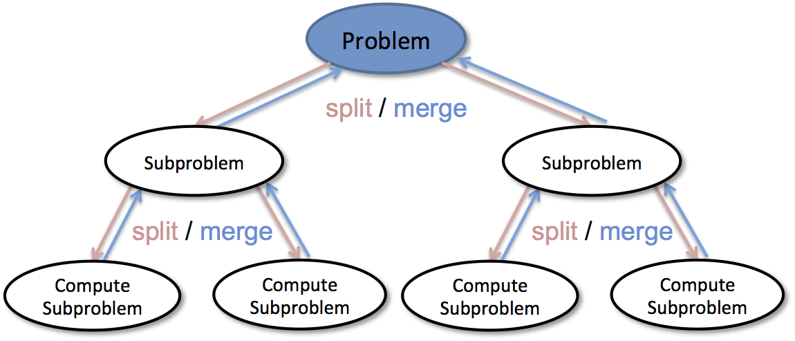
                                                            int binsearch(int arr[],int val,int size)
{
    int low=0;
    int high=size-1;
    for(;low<=high;)
    {
        int mid=(low+high)/2;
        if(arr[mid]==val)
        {
            return mid;
        }
        else if (arr[mid]>val)
        {
            high =mid-1;
        }
        else
        {
            low=mid+1;
        }
    }
    return -1;
}
POPULAR ALGOS
BINARY SEARCH:
This algorithm helps us to immensely reduce the time required to find an object in a sorted array .
Here you maintain 2 pointers one low and another high , pointing at the starting and at the end of the array . Then you take the middle element of the range and check with the value you need to find and 3 cases arise .
The value is equal so you just return the index .
The value is greater so you ignore the right half .
The value is smaller so you ignore the left half .
Time complexity : O(log(n)) .
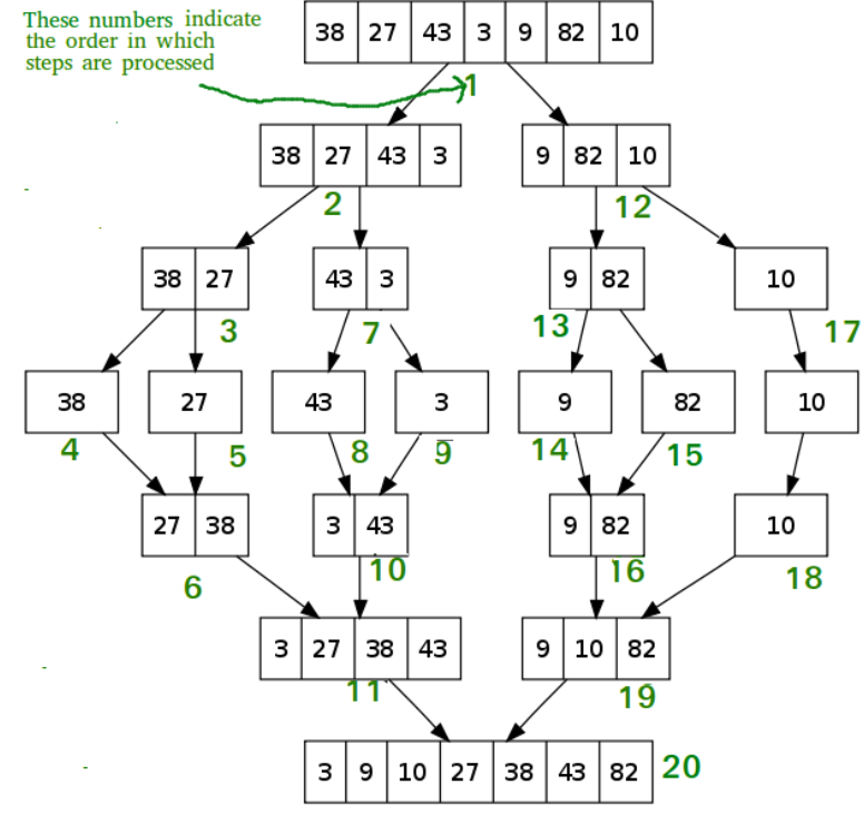
Merge Sort:
This also uses a Divide and Conquer approach . What this algorithm does is first divides the array into two separate halves and sorts them separately and then uses a different merge function to merge the two sorted arrays into a single sorted array . You would get better clarity if you see the figure below .
The base case for this algorithm is when you have a single element in the array and obviously an array of a single element is already sorted .
The Recurrence relation for finding the time complexity is
T(n) = 2T(n/2) + θ(n) .
Which gets solved to T(n)= O(nlogn) .
                                                        void merge(int arr[],int low,int high)
{
   int mid=(low+high)/2;
   int arr1[mid-low+1];//low to mid
   int arr2[high-mid];//mid+1 to high
   for(int i=low;i<=mid;i++)
   {
       arr1[i-low]=arr[i];
   }
   for(int i=mid+1;i<=high;i++)
   {
       arr2[i-mid-1]=arr[i];
   }
   int pt1=low;
   int pt2=mid+1;
   int pt3=low;
   for(;pt1<=mid&&pt2<=high;pt3++)
   {
       if(arr1[pt1-low]<=arr2[pt2-mid-1])
       {
           arr[pt3]=arr1[pt1-low];
           pt1++;
       }
       else
       {
           arr[pt3]=arr2[pt2-mid-1];pt2++;
       }
   }
   for(;pt1<=mid;pt3++,pt1++)
   {
       arr[pt3]=arr1[pt1-low];
   }
   for(;pt2<=high;pt3++,pt2++)
   {
       arr[pt3]=arr2[pt2-mid-1];
   }
}
void mergesort(int arr[],int low,int high)
{
   if(low==high)
   {
       return ;
   }
   int mid=(low+high)/2;
   mergesort(arr,low,mid);
   mergesort(arr,mid+1,high);
   merge(arr,low,high);
}
Study Material for Divide and Conquer
Practice Problem 5
Practice Problem 6
Youtube Video on Divide and Conquer 1
Youtube Video on Divide and Conquer 2
Modular Exponentiation
Modular Exponentiation
A small problem:
You are required to find the remainder of ( 2^20 )%5 .
Very easy right? You might have written something like this
int remainder = ( pow( 2, 20 ) % 5) ;
That's well and good but try outputting ( 2^205 ) with the pow function and you would see something really weird .
The output would show ( -2147483648 ) but that's not correct and how can we find the remainder if the value itself is wrong .
The answer comes with modular exponentiation .
RULES FIRST :
The Rules of modular arithmetic are pretty similar to that of Normal Arithmetic. The only important formula required to learn this concept is
(a*b)%M=( (a%M)*(b%M) )%M
For example : ( 2 *7 )%5=(14%5)=( (2%5)* (7%5) )%5=(22)%5=4
Approach:
So let’s define a function “ MOD(x , n , m) " where this function will give us our desired answer .
So by studying the above mentioned formula we will encounter three different cases . They are as follows :
1. MOD( x ,n ,m )=(MOD(x,n/2,m)MOD(x,n/2,m))%m -------[ if n is even]
2. MOD(x,n,m)=(xMOD(x,n-1,m))%m -------[ if n is odd ]
3. MOD(X,0,M) =1 -------[ if n = 0 ]
                                                            long long MOD(long long x , long long n , long long m)
{
    if(n==0)
    {
        return 1;
    }
    if(n%2==1)
    {
        return (MOD(x,n-1,m)*x)%m;
    }
    else
    {
        long long res = MOD(x,n/2,m);
        return (res*res)%m;
    }

}
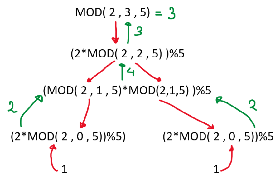
Study Material for Modular Exponentiation
Modular exponentiation (Youtube Reference)
Fast Exponentiation (Youtube Reference)
Practice Problem 3
Practice Problem 4
Matrix Exponentiation
Matrix Exponentiation
Matrix Exponentiation is actually a concept borrowed from Mathematics.
It is a widely used method for solving linear recurrences in an efficient manner.
Some Prerequisites for Matrix Exponentiation :
● Binary exponentiation
● Basic knowledge about matrices
● Recurrence Relations.
Sometimes we might face some problems, where we can easily derive a recursive relation (mostly suitable for dynamic programming approach),but solving with the same linearly might give us TLE, for large values of N(when we have to find the Nth term of the relation). That is where Matrix Exponentiation comes into play.!
A linear recurrence relation is a function or a sequence such that each term is a linear combination of previous terms. Each term can be described as a function of the previous terms. Linear means that the previous terms in the definition are only multiplied by a constant (possibly zero) and nothing else.
Lets Exemplify the same with the classic example of Fibonacci numbers:
We know,
Fib(i)=Fib(i-1)+Fib(i-2).... - for the ith term of the Fibonacci series,with Fib(1)=1,Fib(2)=1. The basic idea behind matrix exponentiation, is to use the base cases of the recurrence relationship in order to assemble a matrix which will allow us to compute values fast.
Let ‘k’ be the number of previous terms on which Fib(i) depends.For example, k=2 in the case of Fibonacci numbers.
Step 1 : Write the recurrence relation as a linear combination of previous k terms with constant coefficients:
F(i)=c1*F(i-1)+c2*F(i-2)+c3*F(i-3)+.. ck*F(i-k),where ci ∈ R
Notice that if we take k=2, and c1=1,c2=1.. Then we get the relation for the Fibonacci sequence.
Step 2 : Now we need to make the relation in a matrix form, so that the Recurrence relation could be satisfied.We would be using the following matrix relation to apply the same :
Fib(i)=T * Fib(i-1)
Here, Fib(i),Fib(i-1) is the matrix used to define the recurrence relation for the ith and (i-1)th terms resp., and T is called the Transformation Matrix.
Obviously, Fib(i) and Fib(i-1) would be represented using the previous k terms.
So, we define Fib(i) as below:
This is the matrix denoting our Fib(i). of order k x 1
Similarly our Fib(i-1) would be of order k x 1.
Therefore our matrix T would be of order k x k.
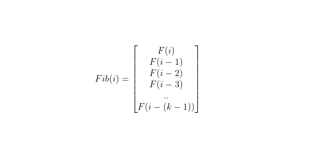
Step 3: This is the most important step in solving recurrence relation.
In this step we would be finding the Transformation Matrix. We know the following points to deduce the T matrix:
● The order of T is k x k
● We have a recurrence relation connecting Fib(i) with k previous terms.
So, the transformation matrix can be represented as::
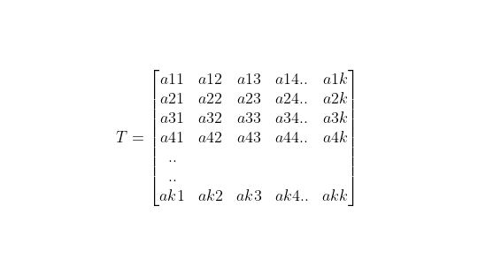
The complete relation can be represented as: Fib(i)= T x Fib(i-1)
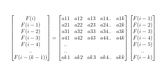
So,here, For the first row, after multiplication we get:
F(i)=a11*(F(i-1))+a12*(F(i-2))+a13*(F(i-3)).. +a1k*(F(i-k))
Comparing this with the Recurrence relation:
F(i)=c1*F(i-1)+c2*F(i-2)+c3*F(i-3)+..ck*F(i-k),where ci ∈ R
Hence, we observe that a11=c1, a12=c2, a13=c3, a14=c4… a1k=ck
Multiplying the second term row of T,
F(i-1)=a21*(F(i-1))+a22*(F(i-2))+a23*(F(i-3)).. +a2k*(F(i-k))
So, we can clearly observe that a21=1, and all other coefficients would be 0.
F(i-1)=1*F(i-1)+0*F(i-2)+... 0*F(i-k)
Similarly,
F(i-2)=0*F(i-1)+1*F(i-2)+0*F(i-3)+... 0*F(i-k).
So, the Transformation Matrix turns out as:
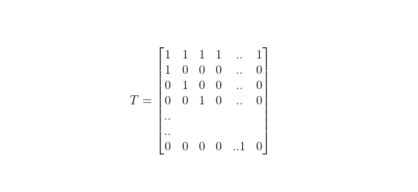
Step 4:Determine Fib(n)
After we construct the transformation matrix, the rest is very simple. We can obtain Fib(i) for any i, by repeatedly multiplying T with Fib(i-1). For example, to obtain Fib(2),
Fib(2)=T*Fib(1)
For Fib(3):
Fib(3)=T*Fib(2)=T2*Fib(1)
Similarly,
Fib(n)=Tn-1*Fib(1)
The only thing which is left for us to perform is calculating Tn-1 efficiently.For calculating TN-1, we can use Binary Exponentiation to solve it in O(Log(N)) time.
Sample code for Nth Fibonacci Series using Matrix Exponentiation:
                                                        //Program to print Nth fibonacci number Modulo 1000000007 using Matrix Exponentiation

#include<bits/stdc++.h>
using namespace std;
#define ll long long
#define MOD 1000000007

ll powM(ll x,ll y,ll m)
{
    ll ans=1,r=1;
    x%=m;
    while(r>0&&r<=y)
    {
        if(r&y)
        {
            ans*=x;
            ans%=m;
        }
        r<<=1;
        x*=x;
        x%=m;
    }
    return ans;
}
void Miden(ll **p1,ll n)
{
    ll (*x)[n]=(ll(*)[n]) p1;
    for(int i=0;i<n;i++)
    {
        for(int j=0;j<n;j++)
        {
            x[i][j]=0;
        }
        x[i][i]=1;
    }
    return;
}
void Mmult(ll **p1,ll **p2,ll **ans,ll x,ll y,ll z,ll m)
{
    ll (*a)[y]=(ll (*)[y])p1;
    ll (*b)[z]=(ll (*)[z])p2;
    ll (*c)[z]=(ll (*)[z])ans;
    for(int i=0;i<x;i++)
    {
        for(int j=0;j<z;j++)
        {
            c[i][j]=0;
            for(int k=0;k<y;k++)
            {
                c[i][j]+=a[i][k]*b[k][j];
                c[i][j]%=m;
            }
        }
    }
    return;
}
void Mpow(ll **p1,ll **ans,ll n,ll y,ll m)
{
    if(y==0)
    {
        Miden(ans,n);
        return;
    }
    ll t[n][n];
    Mpow(p1,(ll **)t,n,y/2,m);
    ll z[n][n];
    Mmult((ll **)t,(ll **)t,(ll **)z,n,n,n,m);
    if(y%2)
    {
        Mmult((ll **)z,p1,ans,n,n,n,m);
    }
    else
    {
        Miden((ll **)t,n);
        Mmult((ll **)z,(ll **)t,ans,n,n,n,m);
    }
    return;
}
int main(){

	ll n;
	cin>>n;
	ll mat[2][2]={{1,1},{1,0}};
	ll ans[2][2];
	Mpow((ll **)mat,(ll **)ans,2,n,MOD);
	cout<<(ans[1][0]*1+ans[1][1])%MOD;

	return 0;
}
Study Material for Matrix Exponentiation
Matrix Exponentiation - Hackerearth Reference
Matrix Exponentiation - GFG Reference
Matrix Exponentiation - Reference
Practice Problem 1
Game Theory
Combinatorial Game Theory
Introduction:
Combinatorial games are two person games with perfect information and no chance moves (no randomization like coin toss is involved that can affect the game). These games have a win-or-lose or tie outcome and are determined by a set of positions, including an initial position, and the player whose turn it is to move. Play moves from one position to another, with the players usually alternating moves, until a terminal position is reached. A terminal position is one from which no moves are possible. Then one of the players is declared the winner and the other the loser. Or there is a tie (Depending on the rules of the combinatorial game, the game could end up in a tie. The only thing that can be stated about the combinatorial game is that the game should end at some point and should not be stuck in a loop.
Let's see an Example:
Consider a simple game which two players can play. There are N coins in a pile. In each turn, a player can choose to remove one or two coins.
The players keep alternating turns and whoever removes the last coin from the table wins.
If N=1 then?
If N=2 then?
If N=3 then?
If N=4 then?
If N=5 then?
If N=6 then?
Once you start playing this game, you will realise that it isn't much fun. You will soon be able to devise a strategy which will let you win for certain values of N. Eventually you will figure out that if both players play smartly, the winner of the game is decided entirely by the initial value of N.
Strategy:
Continuing in this fashion, we find that the first player is guaranteed a win unless N is a multiple of 3. The winning strategy is to just remove coins to make N a multiple of 3.
Finders Keepers game:
A and B playing a game in which a certain number of coins are placed on a table. Each player picks at least 'a' and atmost 'b' coins in his turn unless there are less than 'a' coins left in which case the player has to pick all those left.
(a) Finders-Winners: In this format, the person who picks the last coin wins. Strategy is to reduce the opponent to a state containing (a + b) x k coins which is a losing state for the opponent.
(b) Keepers-Losers: In this format, the person who picks the last coin loses. Strategy is to reduce the opponent to a state containing (a + b) xk + x coins (x lies between 1 and a, both inclusive) which is a losing state for the opponent.
EXAMPLES:
1) A and B play a game of finder-winners with a = 2 and b = 6. If A starts the game and there are 74 coins on the table initially, how many should A pick? If A picks 2, B will be left with 72 and no matter what number B picks, A can always pick (8 - x) and wrap up.
2) A and B play Finders-winners with 56 coins, where A plays first anad a = 1, b = 6. What should B pick immediately after A? A will lose in any case. But the number of coins B picks depends on what A picks.
3) In a game of Keepers-losers played with 126 coins where A plays first ans a = 3, b = 6, who is the winner? In order to win, A should leave 9k+1, 9k + 2 or 9k + 3 coins on the table, since he can do it by picking 6 coins and hence can win the game.
4) In an interesting version of game B gets to choose the number of coins on the table and A gets to choose the format of the game it will be as well as pick coins first. If B chooses 144 and a = 1, b = 5 which format should A choose in order to win? A should choose Keepers-losers and pick 5 coins from the table, leaving 139 coins for B
Properties of the above Games:
1. The games are sequential. The players take turns one after the other, and there is no passing.
2. The games are impartial Given the state of the game, the set of available moves does not depend on whether you are player 1 or player.
3. Chess is a partisan game (moves are not the same).
4. Both players have perfect information about the game. There is no secrecy involved.
5. The games are guaranteed to end in a finite number of moves.
6. In the end, the player unable to make a move loses. There are no draws. (This is known as a normal game, if on the other hand the last player to move loses, it is called a misere game).
Impartial games can be solved using the Sprague Grundy theorem which reduces every such game to Game of NIM.
GAME OF NIM
Given a number of piles in which each pile contains some numbers of stones/coins. In each turn, a player can choose only one pile and remove any number of stones (at least one) from that pile. The player who cannot move is considered to lose the game (ie, one who takes the last stone is the winner).
SOLUTION:
Let n1, n2, ...nk be the sizes of the piles. It is a losing position for the player whose turn it is if and only if n1x or n2x or … x or nk = 0.
Nim-sum: The cumulative XOR value of the number of coins/stones in each pile/heap at any point of the game is called Nim Sum at that point.
If both A and B play optimally i.e they don't make any mistakes, then the player starting first is guaranteed to win if the Nim Sum at the beginning of the game is nonzero. Otherwise, if the Nim Sum evaluates to zero, then player A will definitely lose.
Why does it work?
From the losing positions we can move only to the winning ones:
If x or of the sizes of the piles is then it will be changed after our move (at least one 1 will be changed to 0, so in that column will be an odd number of 1s).
From the winning positions it is possible to move to at least one losing:
If xor of the sizes of the piles is not 0 we can change it to 0 by finding the leftmost column where the number of 1s is odd, changing one of them to 0 and then by changing 0s or 1s on the right side of it to an even number of 1s in every column.
From a balanced state whatever we do, we always end up in an unbalanced state. And from an unbalanced state we can always end up in atleast one balanced state.
Now, the pile size is called the Grundy number of that state.
SPRAGUE-GRUNDY THEOREM
A game composed of K solvable subgames with Grundy numbers G1, G2, ... Gk is winnable if the Nim game composed of Nim piles with sizes G1, G2 ... GK is winnable.
So, to apply the theorem on arbitrary solvable games, we need to find the Grundy number associated with each game state. But before calculating Grundy Numbers, we need to learn about another term - Mex.
What is Mex Function?
'Minimum excludant' a.k.a 'Mex' of a set of numbers is the smallest non-negative number not present in the set.
Eg S = {1, 2, 3, 5}
Mex(S) = 0
S1 = {0, 1, 3, 4, 5}
Mex(S1) = 2
                                                            int calculateMex(set <int> Set)
{
int Mex = 0;
while (Set.find(Mex) != Set.end())
Mex++;
return (Mex);
}
// A function to compute Grundy Number of 'n
//Only this function varies according to the game
int calculateGrundy (int n)
{
if (n == 0)
return (0);
set <int> Set; // A Hash Table
for (int i = 1; i <= n; i++)
Set.insert(calculateGrundy (n-1));
return (calculateMex (Set));
)
Calculating Grundy Numbers
1. The game starts with a pile of n stones, and the player to move may take any positive number of stones. Calculate the Grundy Numbers for this game. The last player to move wins. Which player wins the game?
Grundy (0) = ?
Grundy (1) = ?
Grundy (n) = Mex (0, 1, 2, ....n-1) = n
                                                            int calculateMex(set <int> Set)
{
int Mex = 0;
while (Set.find(Mex) != Set.end())
Mex++;
return (Mex);
)
// A function to Compute Grundy Number of 'n'
// Only this function varies according to the game
int calculateGrundy(int n)
{
if (n == 0)
return (0);
if (n == 1)
return (1);
if (n == 2)
return (2);
if (n == 3)
return (3);
set <int> Set; // A Hash Table
for (int i = 1; i <= 3; i++)
Set.insert(calculateGrundy (n - i));
return (calculateMex(Set));
)
2. The game starts with a pile of n stones, and the player to move may take any positive number of stones upto 3 only. The last player to move wins. Which player wins the game? This game is 1 pile version of Nim.
Grundy (0) = ?
Grundy (1) = ?
Grundy (2) = ?
Grundy (3) = ?
Grundy (4) = mex (Grundy (1), Grundy (2), Grundy (3))
                                                            int calculateGrundy (int n)
{
if (n == 0)
return (0);
set <int> Set; // A Hash Table
Set.insert(calculateGrundy (n/2));
Set.insert(calculateGrundy (n/3));
Set.insert(calculateGrundy (n/6));
return (calculateMex(Set));
}
3. The game starts with a number-'n' and the player to move divides the number-'n' with 2, 3 or 6 and then takes the floor. If the integer becomes 0, it is removed. The last player to move wins. Which player wins the game?
How to apply Sprague Grundy theorem?
Break the composite game into sub-games.
Then for each sub-game, calculate the Grundy Number at that position.
Then calculate the XOR of all the calculated Grundy Numbers.
If the XOR value is non-zero, then the player who is going to make the turn (First Player) will win else he is destined to lose, no matter what.
EXAMPLE PROBLEM:
QCJ3
Tom and Hanks play the following game. On a game board having a line of squares labelled from 0,1,2... certain numbers of coins are placed with possibly more than one coin on a single square. In each turn a player can move exactly one coin to any square to the left i.e, if a player wishes to remove a coin from square 1, he can then place it in any square which belongs to the set (0,1, ... i-1). The game ends when all coins are on square 0 and the player that makes the last move wins. Given the description of the squares and also assuming that Tom always makes the first move you have to tell who wins the game (Assuming Both play Optimally).
(http://www.spoj.com/problems/QCJ3/)
Hint: Each stone at position P, corresponds to a heap of size P in NIM Now, if there are x stones at position n, then n is XORed x times because each stone corresponds to a heap size of n. Then we use the property of xor operator
                                                        #include<iostream>
using namespace std;
int main()
{
int n;
cin>>n;
while(n--)
{
int s;
cin>>s;
long r=0;
int x;
for(int i = 1;i <= s ;i++)
{
cin>>x;
if(x&1)
r=r^i;
		}
cout<<(r == 0? "Hanks Wins" : "Tom Wins")<<endl;
}
return 0;
}
Study Material for Game Theory
LEVEL-5: EXPERIENCED
Graphs and Graph Algorithms (Basic)
Graph terminology
What is a Graph:
In theoretical Computer Science and Discrete Mathematics, a graph is a set of points(vertices) that may or may not contain data connected by a set of lines(edges), which again may or may not contain data.
A Graph may look like this.
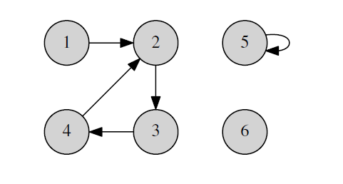
The graph above doesn’t have data stored inside the edges. But some other graphs may have.
The lines can be visualized as “relationships” between any two vertices.
Vertices are often referred to as nodes in a graph.
Terms Used in Graphs:
Since we will be dealing with many complex methods on graphs in further, we need to define some basic terms which we will use there.
1. Node:
A node is basically a point or a circle (it may be represented as some other shape as well). It is the fundamental unit from which a graph is made of. A node can contain data as per requirement.
2. Degree:
Degree is defined for some node in a graph. The degree of a particular node is the number of edges incident on that node.
3. Adjacency:
Adjacency is a property satisfied by two nodes. Two nodes satisfy this property if they are adjacent. Two nodes are adjacent if and only if there is an edge connecting them. Adjacent nodes are also termed as neighbors.
4. Edge:
An edge is represented as a straight line that connects two nodes. This line may represent a unidirectional or bidirectional connection. We draw a simple line for bidirectional connection and a line with an arrow symbol on one of the ends for a unidirectional connection. A unidirectional edge is also termed as a directed edge, and a bidirectional edge is termed as undirected edge.
5. Multiple Edges:
A graph is said to have multiple edges if there exist some pairs of nodes such that there are more than one edges that connect these two nodes. In case of directed edges, there has to be more than one edge that connects the first node to the second node or vice versa. These edges are also called parallel edges.
6. Path :
A path is a sequence of one or more edges that, if followed, will take us from one node to some other node in the graph. The sequence of edges hence formed has to be connected. In other words, for any two adjacent edges in the path, there should be a node in the graph such that the first edge is an incoming edge for it and the second edge is an outgoing one. The number of edges in the path is the length of the path. In a graph with additional information on the edges (or weights), the path length(weight) may be considered as the sum of lengths(weights) of edges involved in the path.
7. Cycle:
A cycle is a path that begins and ends on the same node. A cycle of length one is called a loop (i.e a node connected to itself).
Visualization of Graphs:
Understanding graphs by theoretical definitions may be difficult at times.
So here is a simple explanation that would help you understand graphs.
Consider the following connection of different cities by roads.
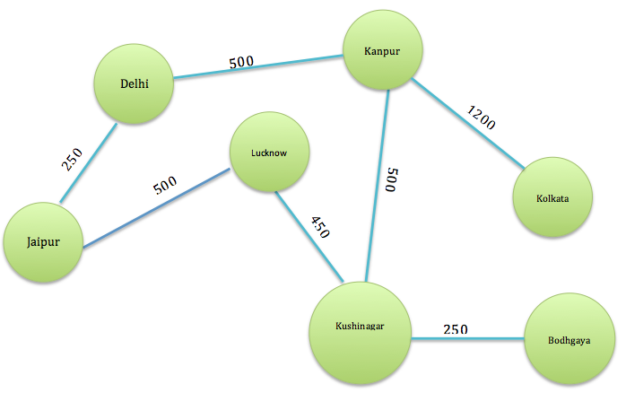
All the cities can be considered as nodes and the roads connecting them as edges. All nodes have data that represents the name of the city. All edges have data that represents the length of the road.
A path from one city to another city(one node to another node) is a connected sequence of roads(edges). The length of a path is the number of roads(edges) in it. And the distance between two cities(nodes) is the sum of the lengths of roads involved in the path connecting these cities.
All the roads(edges) are two-way (bidirectional/undirected) in this graph.
If some road is one way only, we may need to provide additional data about the direction of the roads (usually represented as an arrow).
Study Material for Graph Terminology
Types of Graphs
Classification of graphs
Graphs can be classified in many aspects.
Here a few very common classifications of Graphs:
1. Null Graph :
Graphs having no edges are termed as Null Graphs. A null graph with just one vertex is called a Trivial Graph.
2. Connected and Disconnected Graph:
A graph in which for every node, it is possible to reach every other node by following a valid path, is called Connected Graph. If this property is not satisfied for at least one node, the graph is called Disconnected Graph. A simple example is shown below.
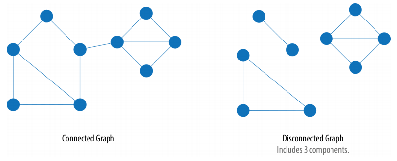
3. Complete Graph:
A graph in which every node is adjacent to every other node is called a complete graph. A complete graph has an edge between every pair of vertices and hence it is possible to reach a vertex from every other vertex by following a path of length one. Here are a few examples of complete graphs. A complete graph for a number of nodes is always unique.
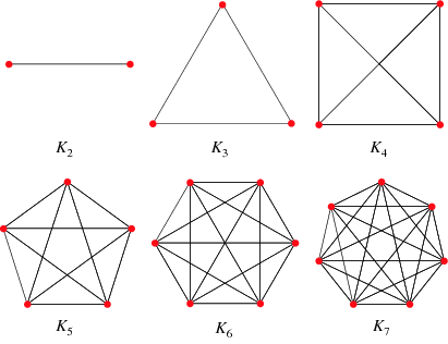
4. Directed Graph:
Graphs having directed edges are called directed graphs.
In other words, The relationship between any two nodes is unidirectional. A simple example is a one-way road. A directed graph is often referred to as a Digraph.
5. Undirected Graph:
Graphs having simple/undirected edges are called undirected graphs. A connection between any two nodes is bidirectional in nature. A simple example is a two-way road.
Unless mentioned, a graph is by convention considered as undirected.
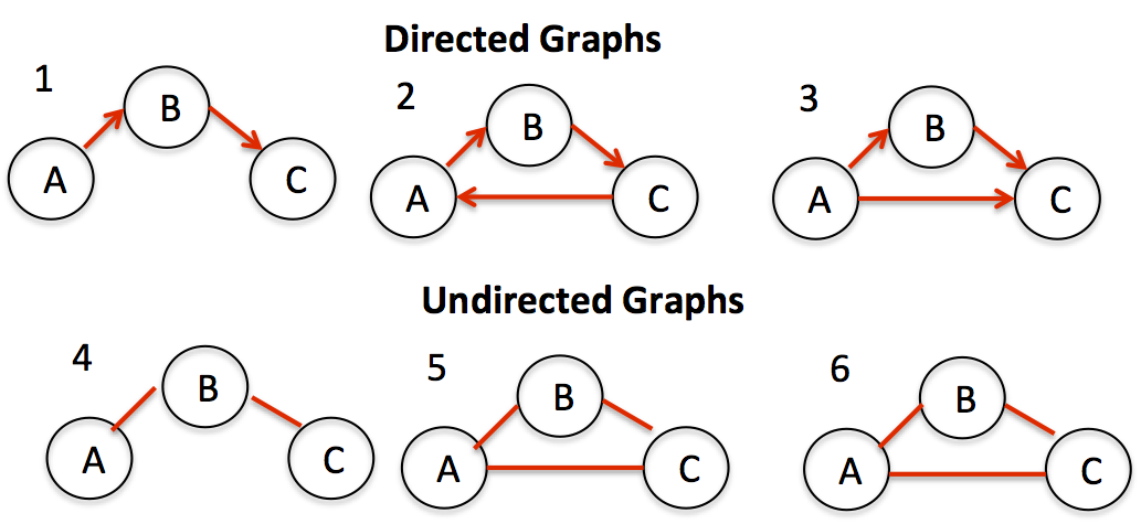
6. Weighted and Unweighted Graphs:
A weighted graph is a graph that has data present on the edges, whereas an unweighted graph doesn’t.
7. Simple Graph:
A simple graph is also called a strict graph. A simple graph is an unweighted undirected graph with no loops or multiple edges.
8. Multigraph:
A graph having multiple edges and self-loops is called a Multi Graph.
9. Tree :
A tree is a connected, acyclic, and undirected graph. The tree is a very special variant of graphs. In a tree, the path from a node to any other node is unique. In a tree with n nodes, the number of edges is always equal to n-1.
10. Sub Graph :
A subgraph of some graph(parent) is defined as a graph whose vertices and edges are a subset of the parent graph.
11. Spanning and Induced Subgraph :
A spanning subgraph of some graph(parent) is a subgraph, which consists of all the vertices of the parent graph.
And an induced subgraph is the one having all the edges of the parent graph.
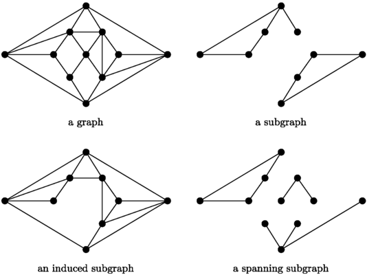
12. Spanning Tree :
A spanning tree of a graph is a spanning subgraph which is also a tree.
A spanning tree of a weighted graph, which has a minimum total weight of edges is also called Minimum Spanning Tree.
13. Bipartite Graph :
A bipartite graph is a graph in which it is possible to divide the vertices into two disjoint sets U and V such that every edge in the graph connects a vertex in U with a vertex in V and no edge connects a vertex to another vertex in the same set.
If for a vertex in a particular set, there is an edge connecting it with every vertex in the other set, then this bipartite graph is called Complete Bipartite Graph. A complete bipartite graph looks like the following.

Study Material for Types of Graphs
Graph Representation
Representation of Graphs
By now, we know that graphs are a collection of vertices and edges. But we have not seen how we can store and use them as a data type. There are different ways to optimally represent a graph, depending on the density of its edges, type of operations to be performed, and ease of use.
In General Programming, we have two major types of representations of graphs.
1. Adjacency Matrix Representation.
2. Adjacency List Representation.
We need these representations in order to store graphs in computer memory.
Adjacency Matrix Representation:
In this type of representation, we use a nXn matrix to store the information about the edges of the graph. The nXn matrix provides us a place to store all possible edges (which indeed are equal to n2) between n nodes.
More formally -
Adjacency Matrix representation is a sequential representation.
It is used to represent the information about two nodes that have an edge between them.
In this representation, we have a nXn matrix, where if we have an edge from node i to node j, then the element in the ith row and jth column is 1 and otherwise 0. In the case of weighted graphs, we can also store the value of the weight of the edge in that matrix element.
For example, the graph shown below can have a matrix representation that looks like the one given on its right.
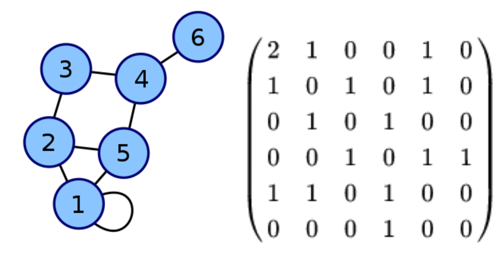
For a weighted graph, the representation looks like this -

Implementation of Adjacency Matrix Representation (in c++)
In c++, the adjacency matrix representation of graphs is done by using a 2-Dimensional Array of size nXn, where n is the number of nodes in the graph.
int adj[n+1][n+1]; // n+1 for 1-indexing
After declaring the matrix (or 2-D array), once we receive any information about an edge, we simply add it to the matrix.
Let say, we have m edges in our graph, and each edge is given input in this format,
a b
Where a and b are the node numbers of nodes that are the endpoints of this edge. So, the code for matrix filling would look like.
                                                            for(int i=1; i<=m; i++)
{
     int a,b;
     cin>>a>>b;
     adj[a][b] = 1;    //If the graph is weighted,
     // let say w is the weight of thisedge,
     // so we write adj[a][b] = w;

    adj[b][a] = 1;    //If the graph is directed,
     // we don't consider the edge in opposite direction.
}
Adjacency Matrix representation is really easy to understand and implement. Processing information about an edge becomes easy as we implement complex algorithms on graphs.
The space required to store a graph is O(n2) as we need a matrix of size nXn.
Adjacency List Representations:
We have seen Adjacency List implementation for representing a graph. But as we can notice, the number of edges in a graph may not always be close to n2. In real life implementations and in most of the problems in Competitive Programming, the graphs are sparse. In other words, the number of edges in a graph is close to O(n).
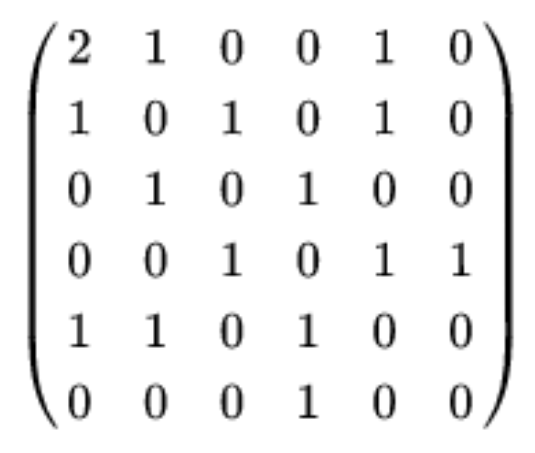
This makes our adjacency matrix representation inefficient because we have so much unused space. Take an example of the adjacency matrix shown above. This matrix has many empty cells, which denotes the unused space.
In order to overcome this memory wastage, we come up with an Adjacency List representation. In this kind of representation, we store the information of some edge between two nodes by linking two memory blocks with each other.
If nodes {n1,n2,n3, . . . ,nt} are connected with node m, then the mth line of the adjacency list will contain these t nodes.
Adjacency List is an array of lists, where the list present at the ith index is the list of nodes that are adjacent or reachable from node i. Below is a visualization of adjacency list.

                                                            for(int i=1; i<=m; i++)
{
       int a,b;
       cin>>a>>b;
       //edge between a and b

       adj[a].push_back(b);
       //there is an edge from a to b

       /*
              For a weighted graph we can have vector<pair<int, int>> adj[N+1];
              Here the first element of the pair will store the adjacent node and the second element will store the weight.
       */

       adj[b].push_back(a);
       // If the graph is undirected
       //there is also an edge from b to a
}
In the case of weighted graphs, we can have additional information about the weight of the edge within the list element.
In C++, dynamically sized containers(vector) are used for representing the list of nodes, hence our adjacency list becomes.
vector<int> adj[N+1]
For weighted graphs, we have to store one extra element of information in the list. So, we can have a list element as a pair to two integers.
vector<pair<int,int>> adj[N+1];
Now, we need to add information about an edge in this list. Let say we have m edges in the graph.
As we can see, the adjacency list stores information of only the edges that are present in the graph, hence drastically reducing the memory space used.
Study Material for Graph Representation
Graph Traversals
Graph Traversals
We already know about representation of graphs and how to store data with help of graphs.
Since graph is a linked data structure, we will now learn how to traverse a graph, or search in a graph.
A graph traversal is a method of visiting each vertex in a graph, starting from a source vertex. The order in which the traversal algorithm visits the nodes in the graph is important and may depend on the problem you are solving. Each vertex is visited exactly once in a traversal algorithm.
There are two major graph traversal algorithms:
Breadth First Search (BFS)
Depth First Search (DFS)
1. Breadth-First Search :
In Breadth-First Search traversal of the graph, we start from a source vertex and we visit all the nodes that are at a distance of one unit from the source, and then we visit all the nodes that are at a distance of two units from the source and then at a distance of three and so on.
This kind of traversal can be visualized as a social network, where we begin from a person (considered to be the source) and then we visit all the friends of this person then we visit all the friends of friends of this person and so on.
Since we will need to have a track of which node to visit first, we will use a
list of nodes yet to be visited and add nodes to this list. Initially, the source node will be added to the list as we begin the depth-first search.
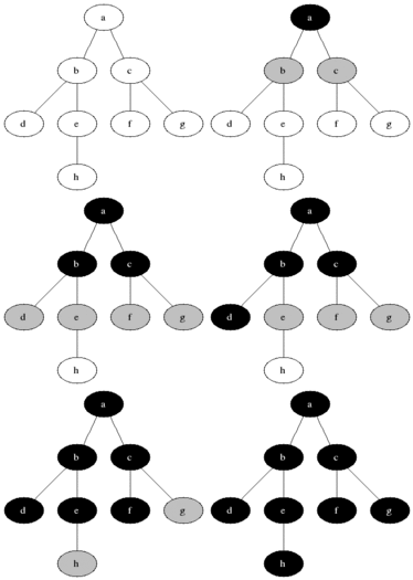
Here is a simple demonstration. Considering a as source vertex,
we will first visit node a. After visiting node a, we will add the adjacents of a, who are b and c into the list of nodes which are
yet to be visited. Then we repeat this process by picking
the first node from the list of friends yet to be visited and adding its adjacents into the list.
For implementation purposes, we use queue data structure to play the role of the list of nodes yet to be visited. So, the algorithm becomes simple.
1. Create a queue of integers to store the node numbers of nodes yet to be visited.
2. Push the source into the queue.
3. While there are some elements in the queue, extract the first element of the queue and store it in some variable say node, currently you are at this node, goto step 4. If the queue is empty, goto step 5.
4. Push all the unvisited adjacents of node into the queue, mark them as visited and goto step 3.
5. Bfs Traversal is completed.
To keep track of already visited nodes, we use an auxiliary array. If the value at ith index of the array is 1, the ith node is visited else no. We initialize this array by 0.
int visited[N+1]={0};
We will use adjacency list representation.
vector<int> adj[N+1];
Here is the implementation for the same.
                                                        void bfs(int source)
{
  queue<int> q;
  q.push(source);
  visited[source]=1;
  // step 1 and 2 complete
  while(!q.empty())
  {
    int node = q.front();
    q.pop();
    //we extract the front node of the queue

    cout<<node<<" "; // we print the node on the screen

    for (int adjacent : adj[node])
    {
      if(visited[adjacent]==0) //we skip all visited adjacents
      {
        visited[adjacent]=1;
        q.push(adjacent);
      }
    }
    // step 4 complete
  }
  // our bfs traversal is complete
}
Analysis of BFS traversal:
Considering |V| as the number of vertices and |E| as the number of edges in the graph.
The time complexity of this algorithm is O(|V|+|E|) as we traverse every vertex and edge at most once.
Auxiliary space required by this algorithm is O(|V|) as the queue can have |V|-1
vertices in it at once in the worst case.
2. Depth First Search:
In Depth First Search of a graph, we start from a source vertex and mark it as visited. Now, we move to its unvisited adjacents one by one and repeat this process. In this way, we traverse the depth of the graph first, rather than traversing the breadth. Here is a simple visualization of the same.
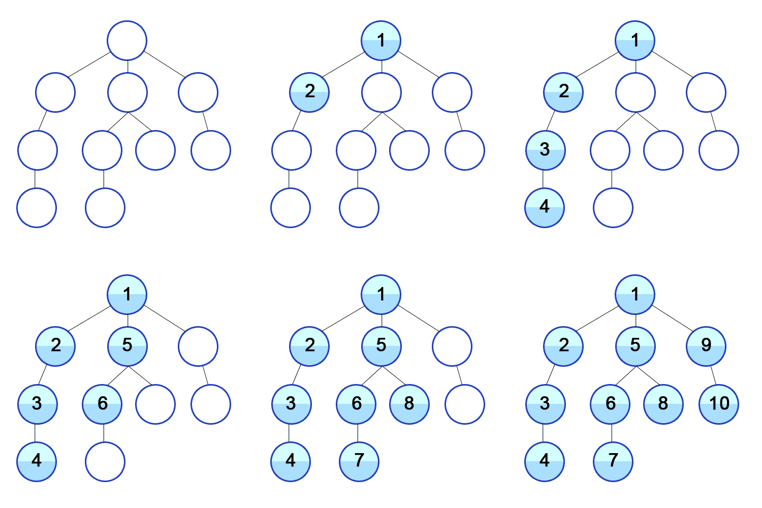
Considering the source vertex as 1, we mark 1 as visited. Now we choose an unvisited adjacent of 1, i.e 2 and visit it and repeat this process for 2. Once we have exited from the dfs of 2, we further move to another unvisited adjacents of 1, i.e. 5 and 9. Note that once we start dfs for a particular node, we first traverse to the whole depth of it and the exit from dfs for that particular node.
This algorithm is conveniently implemented as a recursive algorithm, where we recursively call for dfs function for all unvisited adjacents of the node one-by-one.
The algorithm is as follows.
Let's say that dfs function is called for a particular node.
First, mark this node as visited.
Now iterate over all its adjacents.
If a node is already visited, skip it. Else call dfs for this adjacent.
Once we exit the iteration, the dfs function returns.
We will use an adjacency list representation and a visited array.
vector<int> adj[N+1];
int visited[N+1]={0};
Implementation of DFS.
                                                            void dfs(int source) // step 1
{
  visited[source]=1;
  // step 2 complete

  cout<<source<<" "; // we print the current node on the screen

  for (int adjacent : adj[source]) // step 3
    {
      if(visited[adjacent]==0) //we skip all visited adjacents
      {
        dfs(adjacent);
        // step 4
      }
    }
  // dfs traversal is complete
}
Analysis of DFS traversal:
By convention, taking the number of vertices in this graph as |V| and number of edges as |V|, the time complexity of this traversal is O(|V|+|E|), as we are traversing each vertex and edge once.
Auxiliary Space required by this algorithm is O(h), where h is the maximum height of the graph or the maximum distance of any node from the source. Because of recursive calls, dfs occupies stack memory of the order of O(h).
0-1 BFS
0-1 BFS is a special kind of BFS traversal done on a weighted graph, where the weights on the edges can be one of two values, 0 and 1. And we have to find the weight of the shortest path from source vertex to every other vertex.
A simple example of a 0-1 weighted graph is shown below.
In normal BFS, when we reach a node, we push its adjacent nodes in the back of the queue because they are one level below the current node. But in this case, the nodes having edge weight 0 between them are actually at the same level! So we push those nodes on the front of the queue and that’s it, our 0-1 BFS Algorithm is complete.
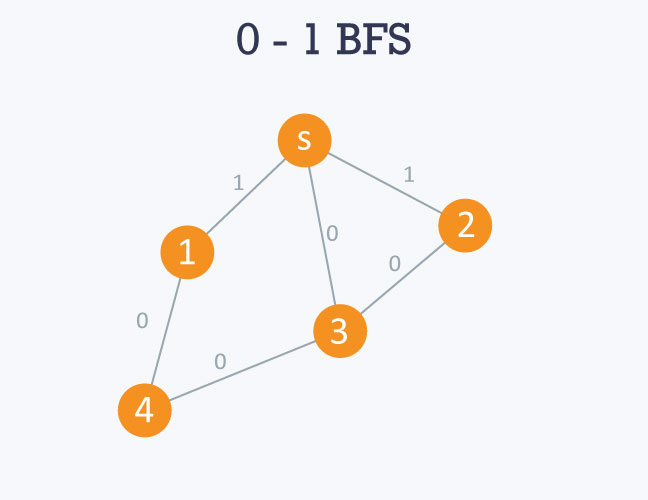
Algorithm
1. Start from a source vertex, push it into the queue and mark it as visited. And its distance is zero.
2. While the queue is not empty, pop a node from the front of the queue and goto step 3. If the queue is empty, goto step 4.
3. For all unvisited adjacents of this node, if the edge weight is 0, push the node in the front of the queue and set the distance of this node as same as distance of the popped node else push it in the back of the queue and set the distance one more than the distance of the popped node. Mark this node as visited and goto step 2.
4. Our 0-1 BFS traversal is complete.
We will use adjacency list representation with weight information and an auxiliary array for keeping track of visited nodes. For the purpose of pushing in front of the queue, we will use a deque data structure, instead of queue data structure. We use another auxiliary array to store the final distance of ith node from the source vertex.
vector<pair<int,int>> adj[N+1];
int visited[N+1]={0};
deque<int> q;
Implementation of 0-1 BFS.
                                                        void zero_one_bfs(int source)
{
  deque<int> q;
  // initialize a double ended queue
  q.push_back(source);
  visited[source]=1;
  // step 1 complete

  while(!q.empty()){ // step 2 begins
    int node = q.front();
    q.pop_front();

    cout<<node<<" "; // we print the node on the screen
    for(pair<int, int> info : adj[node])
    {
      int adjacent = info.first;
      int weight = info.second;
      // extract the adjacency information

      if(visited[adjacent]==0){ // we skip all visited adjacents
        if(weight==0){
          q.push_back(adjacent);
        }
        else {
          q.push_back(adjacent);
        }
        visited[adjacent]=1;
      }
        // step 3 complete
    }
  }
}
Analysis of 0-1 BFS :
This algorithm is no different from a normal BFS algorithm. The key implementation difference is the double-ended queue.
Hence the time complexity of this algorithm is O(|V|+|E|) and space complexity is O(|V|).
Study Material for Graph Traversals
Connected Components & SCCs
Connectivity in Graphs
Graphs are based on connection of several different points with each other. These points are kept on a plane and a line is drawn between any two points to connect them.
Since a very important aspect of a graph is connection, we define the connectivity of a graph as follows.
Connectivity is a basic concept of graph theory, it defines whether a graph is connected or not.
A graph is said to be connected if it is possible to traverse from any vertex to every other vertex by following a sequence of connected edges.
A graph is said to be disconnected if there exists a pair of vertices such that there is no path between them.
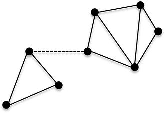
Let’s call the edge, that is shown with dotted lines as E. So, here in this graph, the presence of E makes it possible to traverse from any vertex to every other vertex, by following some sequence of edges. But, if we remove this edge, then it is not possible to traverse from certain points to other points in the graph. In formal words, if edge E is not present in the graph, it is disconnected and connected otherwise.
Let’s now define some terms related to graph connectivity.
1. Connected Component:
A connected component of a graph is a maximal connected subgraph of it. A maximal connected subgraph is a subgraph which cannot be further expanded to include more nodes of it’s parent node. Two connected components of a graph cannot be connected within themselves, in other words, the connected components of a graph are disjoint. The union of all connected components forms, the set of all vertices, i.e. the graph. A connected graph is a connected component of itself.
2. Cut Vertex:
A cut vertex is defined for a connected graph. It is a vertex, removal of which results in the connected graph being disconnected.
3. Cut Edge (Bridge):
A cut Is also defined for a connected graph. It's an edge, the removal of which results in the graph being disconnected.
4. Cut Set:
If deleting a certain number of edges in a graph makes it disconnected then those deleted edges is called a cut set of the graph. The removal of some but not all edges of the cut set does not disconnect the graph.
5. Edge Connectivity:
It is the minimum number of edges whose removal makes it disconnected. In other words it is the minimum size of the cut set of the graph.
6. Vertex Connectivity:
It is the minimum number of vertices that need to be removed from the graph to make it disconnected.
Connected Component Algorithms:
Finding the connected components of a given graph can be done algorithmically. We use normal BFS or DFS traversal to find the connected components of a graph. We need an auxiliary array to keep track of the visited nodes. The algorithm is as follows.
1. Iterate on every node from 1 to N.
2. If the note is visited then skip to the next node. Else go to step 3.
3. Cal DFS or BFS traversal for that particular node and print a new line character.
4. As we exit the iteration, we have counted all connected components of the graph.
We are going to need an auxiliary array to keep track of visited nodes and an adjacency list representation of the graph. We will be using the traverse() function, the internal implementation of which may either be BFS or DFS.
int visited[N+1];
vector<int> adj[N+1];
void traverse(int source);
Here is the implementation.
                                                            for (int node = 1; i < = N; node++) // step 1
{
  if(visited[node]){
    continue;
    // step 2
  }
  traverse(node);
  cout<<"\n";
  // step 3
}
//step 4
Analysis of Connected Components Algorithm
By convention, the number of nodes in the graph is |V| and number of edges is |E|. So, the time complexity of this algorithm is O(|V|+|E|) as all connected components are disjoint and we visit a node and edge exactly once.
If the internal implementation of the traverse() function is BFS algorithm, the space complexity of this algorithm is O(|V|) as, in the worst case the graph can be connected. If the internal implementation is a recursive DFS algorithm, the space complexity will be O(h), where h is the maximum height of any connected component.
Strongly Connected Graph:
The idea of strongly connected components is applicable on directed graphs. A directed graph is said to be strongly connected if there is a path between each pair of vertices in it. The pair of vertices is ordered here, as we know that if there is a path from vertex a to vertex b, there need not be a path from b to a.
In other words, if every vertex is reachable from every other vertex in a directed graph, the graph is strongly connected.
Consider this graph. All vertices can be reached from every other vertex. Hence this is a strongly connected graph.
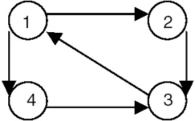
Strongly Connected Components (SCCs):
Just like connected components, strongly connected components are maximal strongly connected subgraphs of a graph.
For example in the graph shown below, the subgraphs enclosed in the colored regions are strongly connected components. We can reach from any vertex to every other vertex in a strongly connected component.
Algorithms for finding Strongly Connected Components:
Kosaraju’s Algorithm
Tarjan’s Algorithm
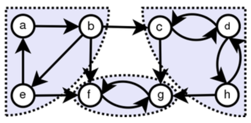
Study Material for Connected Components & SCCs
Kosaraju’s Algorithm
Tarjan’s Algorithm
Component Graph Theory - Wikipedia
Strongly Component Graph Component - Wikipedia
Strongly-Connected-Graphs - Tutorialspoint
Strongly Connected Components - GFG
Practice Problem 1
Practice Problem 2
Cycle Detection
Cycle Detection in graphs
Graphs are a connection of points with help of some lines. Each relation between any two points is independent of the relation between some other pair of points. In such cases, the edges are added independently.
We define a path as a sequence of edges that takes us from a point to another point in the graph. But since the edges are added independently, we can have a path that has a non-zero length and it starts and terminates at the same point. We call this a cycle. The only repeated vertices in the cycle must be the first and the last vertices. Edges should not get repeated.
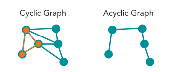
Cycle Detection in Undirected Graphs:
A cycle represents a path that starts and ends at the same vertex. To check if there is a cycle in an undirected graph, we will need to check if we can reach a vertex, starting from another vertex using some path that has no-zero length and doesn’t contain repeating edges.
We can easily achieve this using a simple BFS/DFS traversal algorithm. In each of the above mentioned traversals, we have an auxiliary array that keeps track of already visited nodes. But the question is how we come to know about the existence of a cycle?
The answer is pretty simple. While in the traversal, checking for the adjacent nodes of the node we are currently at, if we encounter a node that is already visited but is not a parent of the current node, this is a cycle! The proof is quite intuitive and simple. Consider a simple path that connects two points in a graph. This path is not a cycle and connects two different points. The only thing that can make this path a cycle is an extra edge between it’s two endpoints. And that is exactly we are searching for. The algorithm is as follows.
Algorithm for cycle detection:
1. Start DFS/BFS traversal from any point in the graph.
2. While searching for unvisited adjacent nodes, if we encounter an already visited node, goto step 3.
3. Check if the node is the parent of the current node. If yes, go back to step 2, else go to step 4.
4. We have found a cycle.
For implementation purposes, we use an adjacency list, an auxiliary array to keep track of visited nodes.
vector<int> adj[N+1];
int visited[N+1];
DFS based algorithm:
In order to check if a node is the parent of some node in that particular traversal, we pass an extra parameter to the dfs function, named as par. This variable will store the information about the parent of the node we are currently at.
DFS based implementation of Cycle Detection Algorithm:
                                                        bool isCyclic(int node, int par){
  // enter the DFS traversal

  visited[node]=1;

  for(int x: adj[node]){
    // check for all adjacent nodes

    if(visited[x]==1){ // as we encounter a visited node
      if(par==x) continue;
      // if the visited node is the parent of this node
      // we can skip it

      // else we have detected a cycle
      return true;
    }
    if(dfs(x,node)) { //if we detect a cycle in DFS call
      // for a child
      return true; // then this DFS call must also return true
    }
  }
  // if no cycle found
  return false;
}
For implementation purposes, we use adjacency list representation, an auxiliary array to keep track of visited nodes, and a queue of pairs to store the information about the parent of each node.
vector<int> adj[N+1];
int visited[N+1];
queue<pair<int,int>> q;
BFS based implementation :
                                                        bool isCycle(int source){
  queue<pair<int, int>> q;

  q.push({source,source}); //we consider the parent of the
  // source node as the source node itself

  while(!q.empty()){
    pair<int, int> p = q.front();
    q.pop();
    int node = p.first;
    int parent = p.second;
    for(int x:adj[node]){  //for all adjacents to the current node

      // if we encounter a visited node
      if(visited[x]){
        //if the node is the parent
        if(x==parent) continue;
        // else we found a cycle
        return true;
      }
      //else we push this node in the queue
      visited[x]=1;
      // the parent of x is node
      q.push({x, node});
    }
  }
  // if we traversed all the nodes and didn't find a cycle
  return 0;
}
Analysis:
Both the BFS and DFS based algorithms have same time complexities as normal BFS and DFS algorithms.
Study Material for Cycle Detection
LEVEL-6: PROFICIENT
Trees
LOWEST COMMON ANCESTOR (LCA)
Given a binary tree and two nodes x and y, find the lowest common ancestor.
What is LCA?
Let x and y be two nodes of the tree T. LCA is defined as the lowest node that has both x and y as descendants. Also, a node can be a descendant of itself.
In the figure given to the right, the lowest common ancestor is shown in dark green. Whereas the light green nodes are the other common ancestor (but not the lowest).
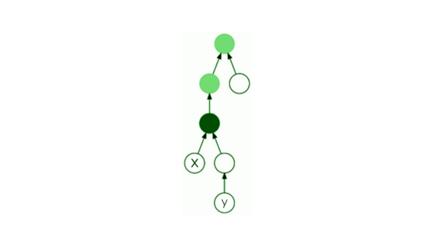
Given below are a few examples:
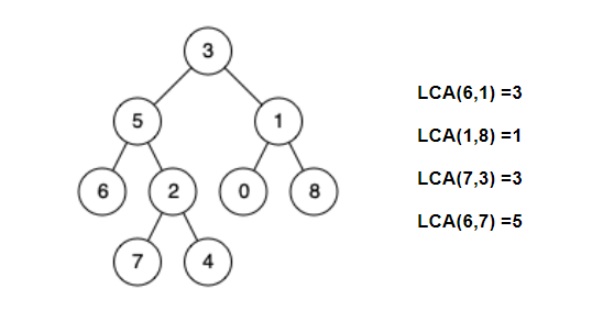
APPROACH:
The main approach is that we recursively search left and right for the two given nodes, i.e. x or y.
If we find either of the nodes, we return the node. Else if we do not find the node in a sub-tree, we return null.
After we are done searching both left and right subtrees of a node, we come across three possibilities:
1. If both left and right are not null – We found the LCA and return the LCA
2. If both left and right are null – We continue our search
3. If either left or right are not null –
● If left is null, return the right node
● If right is null, return the left node
TIME & SPACE COMPLEXITY :
Time Complexity: O(n) [since we traverse all n nodes of the tree]
Space Complexity: O(h) [where h is the maximum height of the tree]
                                                        lca(root, x, y)
{
    //base case
    if (root == null)
    {
        return null;
    }
    if (root == x || root == y)
    {
        return root;
    }

    left = lca(root->left, x, y);
    right = lca(root->right, x, y);

    //case 1
    if (left != null && right != null)
    {
        return root;
    }
    //case 2
    if (left == null && right == null)
    {
        return null;
    }
    // case 3
    if (left != null)
    {
        return left;
    }
    else
    {
        return right;
    }
}
EXAMPLE :
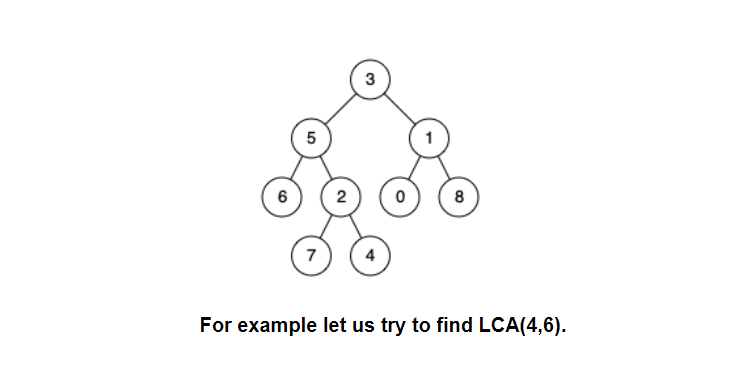
We start from the node having the value 3. Since it is not equal to either 4 or 6, we move to the left subtree (i.e. node 5). The same happens with the node 5 and we move further to the left side (i.e. node 6).
Now we find our first match and the left of node 5 stores node 6. …(a)
Moving to the right subtree of node 5, node 2 is also not equal to 6 or 4. Left of node 2 (i.e. node 7) returns null and right of node 2 (i.e. node 4) returns node 4 since we found out our second match.
Node 2 returns node 4 to the right of node 5. …(b)
Since both the left and right of node 5 are not null [by (a) and (b)], we found the LCA.
The entire tree will be traversed similarly, which will end up giving the final result as LCA(6,4) =5.
Study Material for LCA
MINIMUM SPANNING TREE
In a weighted undirected graph, let’s say there are V vertices and E edges
[ G = ( V,E ) ]. So minimum spanning tree is a subgraph of a graph that is a tree and it connects all the vertices together besides having the least weight (i.e. the sum of weights of edges is minimal).
To get least weight , we want less no of edges. So for all the vertices to get connected, we require minimum (V - 1) edges in overall.
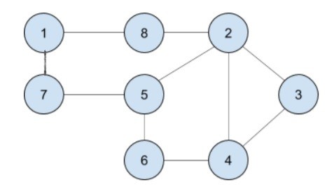

In Fig 1(a), there are 8 vertices and 10 edges and all vertices are connected. Fig 1(b) is a subgraph of graph 1(a) and it has 8 vertices and 7 ( 8 - 1 ) edges and we can clearly see that all vertices are connected with minimum no of edges.
If the above edges were weighted, we had to choose such a path such that the total weight is minimum and edges present in that subgraph is (V-1).
Prim's Algorithm
The minimum spanning tree is built gradually by adding edges one at a time.
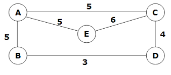
At first the spanning tree consists only of a single vertex (chosen arbitrarily).
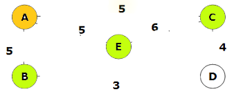
Then the minimum weight edge outgoing from this vertex is selected and added to the spanning tree.
Here, A is chosen and the outgoing weighted edges are 5, 5 and 5. So we can choose any edges since all are same.
After that the spanning tree now consists of two vertices. Now we select the edge which is having the minimum weight and also,it must be outgoing from any of the selected 2 vertices.
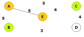
Vertices A and E are already selected and the outgoing weighted edges from A and E are 5 , 6 and 5.
So minimum weight edge is 5. So we can choose any of the two edges with weight 5.
And so on, i.e. every time we select and add the edge with minimal weight that connects one selected vertex with one unselected vertex. The process is repeated until the spanning tree contains all vertices (or equivalently until we have n−1 edges).
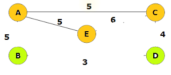
Vertices A, C and E are already selected and the outgoing weighted edges from A, C and E are 5 and 4.
So minimum weight edge is 4.
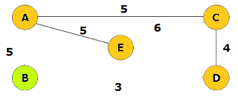
Vertices A, C, D and E are already selected and the outgoing weighted edges from A, C, D and E are 5 and 3.
So minimum weight edge is 3
In the end the constructed spanning tree will be minimal. If the graph was originally not connected, then there doesn't exist a spanning tree, so the number of selected edges will be less than V−1.
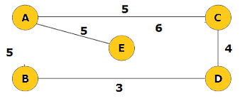
So minimum weight spanning tree is 5 + 5 + 4 + 3 = 17.
Dense graphs: O(n²) [ n : vertices ]
                                                        int n; //no of vertices
vector<vector<int>> adj; // adjacency matrix of graph
const int INF = 1000000000; // weight INF means there is no edge

struct Edge {
    int w = INF, to = -1;
};

void prim() {

    int total_weight = 0;

    vector<bool> selected(n, false); // no vertex selected yet
    vector<Edge> min_e(n);

    min_e[0].w = 0;

    for (int i = 0; i < n; ++i) {

        int v = -1;
        for (int j = 0; j < n; ++j) {

            if (!selected[j] && (v == -1 || min_e[j].w < min_e[v].w))
                v = j;
        }

        if (min_e[v].w == INF)
        {
            cout << "No Minnimum Spanning Tree!" << endl;
            exit(0);
        }

        selected[v] = true;
        total_weight += min_e[v].w;

        if (min_e[v].to != -1)
            cout << v << " " << min_e[v].to << endl;

        for (int to = 0; to < n; ++to) {
            if (adj[v][to] < min_e[to].w)
                min_e[to] = {adj[v][to], v};
        }
    }

    cout << total_weight << endl;
}
Sparse graphs: O(mlogn) [ n : vertices, m : edges ]
                                                        const int INF = 1000000000;

struct Edge {
    int w = INF, to = -1;
    bool operator<(Edge const& other) const {

        return make_pair(w, to) < make_pair(other.w, other.to);
    }
};

int n;
vector<vector<Edge>> adj;

void prim() {
    int total_weight = 0;
    vector<Edge> min_e(n);
    min_e[0].w = 0;
    set<Edge> q;
    q.insert({0, 0});
    vector<bool> selected(n, false);
    for (int i = 0; i < n; ++i) {
        if (q.empty()) {
            cout << "No MST!" << endl;
            exit(0);
        }

        int v = q.begin()->to;
        selected[v] = true;
        total_weight += q.begin()->w;
        q.erase(q.begin());

        if (min_e[v].to != -1)
            cout << v << " " << min_e[v].to << endl;

        for (Edge e : adj[v]) {
            if (!selected[e.to] && e.w < min_e[e.to].w) {
                q.erase({min_e[e.to].w, e.to});
                min_e[e.to] = {e.w, v};
                q.insert({e.w, e.to});
            }
        }
    }

    cout << total_weight << endl;
}
Kruskal's algorithm
Firstly,all edges are sorted by weight (in non-decreasing order).
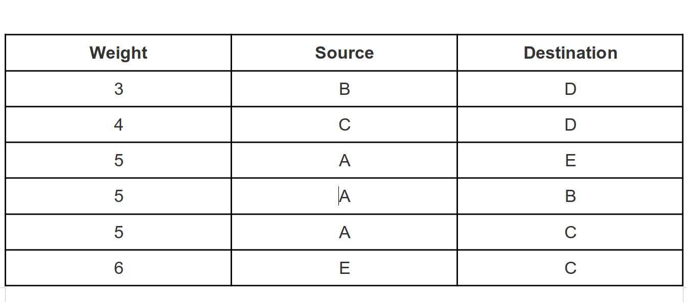
We pick all edges from the first to the last (in sorted order), and if the ends of the currently picked edge belong to different subtrees, these subtrees are combined, and the edge is added to the answer. After iterating through all the edges, all the vertices will belong to the same sub-tree, and we will get the answer.
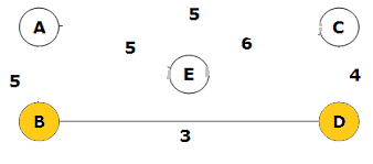
We pick the edge B - D as it contained the minimum weight 3 and is not forming a cycle
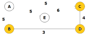
We pick the edge C - D as it contained the next minimum weight 4 and is not forming a cycle too.

We pick the edge A - E and it is not forming a cycle too.
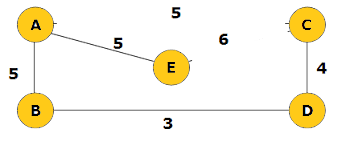
Finally, we pick the edge A - E.
Study Material for Minimum Spanning Tree
Graph and Graph Algorithms (Advanced)
Topological Sorting
Consider the following situation:
There are 10 locks- all possessing a strange property:
A lock might require few other locks to be unlocked before one can unlock it. You have been provided the dependencies of the locks and are asked to unlock all of them.
So, how to find an order to unlock all the locks, or to check if it is impossible to do so?
The kind of technique which should be employed to achieve such an order is termed as Topological Sorting.
In the above example, one approach could be to unlock all the locks firstly which does not depend on any other locks. Now the dependency of a few locks would have been reduced. Those that no longer require any other locks to be unlocked before them, can now be unlocked. We repeat the process until all the locks have been unlocked.
This implementation is similar to that of Kahn’s Algorithm.
Note: It might not always be possible to find a valid unlocking order for the locks.
Prerequisites for Topo(Topological) sort:
Basic knowledge on Graphs
Array Manipulation
(Optional)Knowledge of queue STL
Definition:
A topological sort is an ordering of the nodes of a directed graph such that if there is a path from node a to node b, then node a appears before node b in the ordering. For example, for the graph:
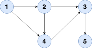
One possible topological order can be : 1,2,4,3,5
Here, every node is placed before a node with an edge directed towards it from that very node.
An acyclic graph always has a topological sort. However, if the graph contains a cycle, it is not possible to form a topological sort, because no node of the cycle can appear before the other nodes of the cycle in the ordering. It turns out that depth-first search can be used to both check if a directed graph contains a cycle and, if it does not contain a cycle, to construct a topological sort!
Algorithm:
The idea is to go through the nodes of the graph and always begin a depth-first search at the current node if it has not been processed yet. During the searches, the nodes have three possible states:
State 0:the node has not been processed.
State 1:th node is under processing.
State 2:the node has been processed.
Initially, the state of each node is 0. When a search reaches a node for the first time, its state becomes 1. Finally, after all successors of the node have been processed, its state becomes 2.
If the graph contains a cycle, we will find this out during the search, because sooner or later we will arrive at a node whose state is 1. In this case, it is not possible to construct a topological sort
If the graph does not contain a cycle, we can construct a topological sort by adding each node to a list when the state of the node becomes 2. This list in reverse order is a topological sort
Hence, we can draw the following conclusions with respect to topological sorting:
•Any node prior to a node after it in the ordering, cannot have a directed edge towards itself from that node.
•Topological sorting is applicable only for acyclic graphs.
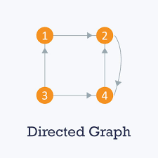
For Example, Topological sort is not applicable for this graph,since there is a cycle in it.
While implementing our algorithm, we take us of the following states:
State 0:The nodes have yet not been visited.
State i -the nodes of this state are under process.
If we encounter any node of the same state while doing a depth first search, we can safely assume that the graph contains a cycle.
Implementation:
                                                            int n; // number of vertices
vector<vector<int>> adj; // adjacency list of graph
vector<int> visited;
vector<int> topo;

bool dfs(int v,int state) {
    visited[v] = state;
    for (int u : adj[v]) {
        if (!visited[u]){
            bool possible=dfs(u,state);
            if(!possible)
                return false;
        }
        else if(visited[u]==state)
            return false;
    }
    topo.push_back(v);
    return true;
}
void topological_sort() {
    visited.resize(n+1);
    topo.clear();
    int state=0;
    bool ok=true;
    for (int i = 0; i < n; ++i) {
        if (!visited[i]){
            ok=dfs(i,state++);
            if(!ok)
                break;
        }

    }
    if(!ok)
        cout<<"The Graph contains at least 1 cycle";
    else{
        reverse(topo.begin(), topo.end());
        for(auto ver:topo)
            cout<<ver<<" ";
    }
}
int main() {
    int m,u,v;
    cin>>n>>m;
    for(int i=1;i<=n;i++){
        cin>>u>>v;
        adj[u].push_back(v);
    }
    topological_sort();

    return 0;
}
Complexity Analysis:
Time Complexity: O(V+E), where V-number of vertices, E-number of edges in the graph.
•The algorithm followed mainly is a DFS, so its complexity is the same.
Space complexity: O(V+E)
•The auxiliary space required is for keeping track of the state of the current operating nodes, and for keeping track of the edges.
Kahn’s Algorithm:
Kahn’s Algorithm is another method for finding Topological sort of a directed acyclic graph(DAG).The algorithm provides an efficient method for finding the topological sort of a graph.
The algorithm works by finding vertices with no incoming edges and removing all outgoing edges from these vertices.
Algorithmic Steps:
The idea is to maintain in-degree information of all graph vertices, by storing them in an array/vector.
In-degree- Count of the number of incoming edges directed towards a vertex.
•The algorithm starts with a vertex having indeg=0.
•The edges directed from this vertex to other nodes are removed, by decreasing their indegrees by 1.
•Processes 1 and 2 are repeated until no vertices with 0 indegree is left.
•If the graph contained a cycle, it would still have edges remaining after the process ends.
Implementation:
                                                            vector<int>topo;
bool Topological_Sort(){
    int n,m,u,v;
    cin>>n>>m;
    vector<int>adj[n+1];
    vector<int>indeg(n+1);
    for(int i=1;i<=n;i++){
        cin>>u>>v;
        adj[u].push_back(v);
        indeg[v]++;
    }
    queue<int>q;
    for(int i=1;i<=n;i++){
        if(!indeg[i])
            q.push(i);
    }
    vector<int>topo;
    while(!q.empty()){
        int node=q.front();
        q.pop();
        topo.push_back(node);
        for(auto child:adj[node]){
            if(indeg[child]==0)
                continue;
            indeg[child]--;
            if(indeg[child]==0)
                q.push(child);
        }
    }
    for(int i=1;i<=n;i++){
        if(indeg[i])
            return false;
    }
    return true;
}
int main() {

    bool isPossible=Topological_Sort();
    if(isPossible){
        for(auto vert:topo)
            cout<<vert<<" ";
    }
    else
        cout<<"The Graph contains at least 1 cycle";

    return 0;
}
Complexity Analysis:
Time Complexity: O(V+E), where V-number of vertices, E-number of edges in the graph.
The algorithm followed mainly is a DFS, so its complexity is the same.
Space complexity: O(V+E)
The auxiliary space required is for storing the edges, and the indegree values.
Study Material for Topological Sorting
Problem 5
Topological Sorting - Competitive Programming Algorithms
Topological Sort Tutorials & Notes | Algorithms
Topological Sorting
Shortest Path Algorithms
Shortest path between two points implies the minimum summation of the edges connecting the given points.
Consider the following situation:
Suppose you are standing in city A, and you have to reach the city Z. Each of the cities named B to Y, have interconnecting passages of varying lengths. The distances are provided to you, but you want to reach Z travelling the shortest path possible.
This is actually a real-life application of shortest distance algorithms.
PREREQUISITES:
Knowledge about the different components of a graph- nodes,edges,weights of a graph.
Knowledge on STL containers like Priority Queue, Multisets, and/or queues,vectors.
Basic array manipulation
Algorithms:
1)Bellman-Ford Algorithm: This Algorithm is used to find the shortest distance from a source vertex to other nodes.
This algorithm uses different edges to reduce the distance of nodes from the vertex until it can no longer be reduced. Initially, the distances are initialised to a maximal value which can possibly not be an ans.(we’ll call it infinity or just inf.).
A very important use of this algorithm is to detect the presence of negative cycles.
Negative Cycles:
If the graph contains a negative cycle, we can shorten infinitely many times any path that contains the cycle by repeating the cycle again and again. Thus, the concept of a shortest path is not meaningful in this situation.
A negative cycle can be detected using the Bellman–Ford algorithm by running the algorithm for n rounds. If the last round reduces any distance, the graph contains a negative cycle. Note that this algorithm can be used to search for a negative cycle in the whole graph regardless of the starting node.
Algorithm steps:
•The outer loop traverses from 0 to n−1
•Loop over all edges, check if the next node distance > current node distance + edge weight, in this case update the next node distance to "current node distance + edge weight".
This algorithm depends on the relaxation principle where the shortest distance for all vertices is gradually replaced by more accurate values until eventually reaching the optimum solution. In the beginning all vertices have a distance of "Infinity", but only the distance of the source vertex = 0, then update all the connected vertices with the new distances (source vertex distance + edge weights), then apply the same concept for the new vertices with new distances and so on.
A diagrammatic representation of Bellman-Ford’s algorithm:
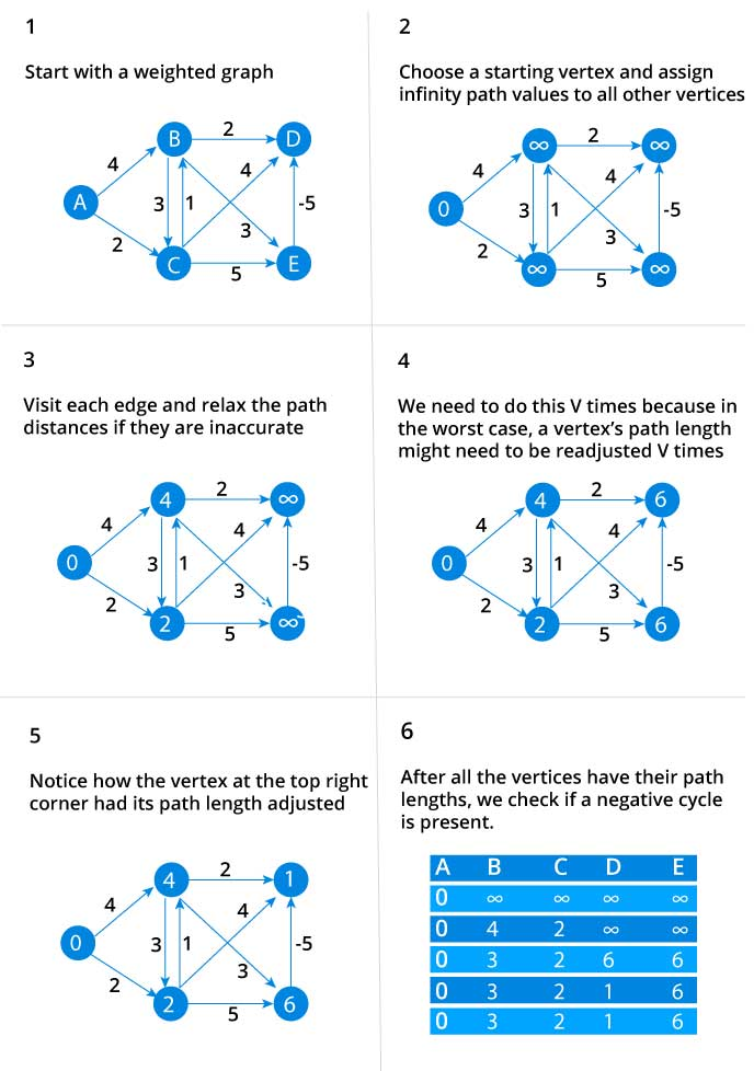
Implementation:
                                                        struct edge
{
    int a, b, cost;
};

int n, m, v;
vector<edge> e;
const int INF = 1000000000;

void solve()
{
    vector<int> d (n, INF);
    d[v] = 0;
    for (int i=0; i<n-1; ++i)
        for (int j=0; j<m; ++j)
            if (d[e[j].a] < INF)
                d[e[j].b] = min (d[e[j].b], d[e[j].a] + e[j].cost);
    // display d, for example, on the screen
}
Shortest Path Faster Algorithm (SPFA)
The SPFA algorithm is a variant of the Bellman–Ford algorithm that is often more efficient than the original algorithm.
The SPFA algorithm does not go through all the edges on each round, but instead, it chooses the edges to be examined in a more intelligent way.
The main idea is to create a queue containing only the vertices that were relaxed but that still could further relax their neighbors. And whenever you can relax some neighbor, you should put him in the queue. This algorithm can also be used to detect negative cycles as the Bellman-Ford.The efficiency of the SPFA algorithm depends on the structure of the graph: the algorithm is often efficient, but its worst case time complexity is still O(nm)
and it is possible to create inputs that make the algorithm as slow as the original Bellman–Ford algorithm.
Implementation:
                                                            const int INF = 1000000000;
vector<vector<pair<int, int>>> adj;

bool spfa(int s, vector<int>& d) {
    int n = adj.size();
    d.assign(n, INF);
    vector<int> cnt(n, 0);
    vector<bool> inqueue(n, false);
    queue<int> q;

    d[s] = 0;
    q.push(s);
    inqueue[s] = true;
    while (!q.empty()) {
        int v = q.front();
        q.pop();
        inqueue[v] = false;

        for (auto edge : adj[v]) {
            int to = edge.first;
            int len = edge.second;

            if (d[v] + len < d[to]) {
                d[to] = d[v] + len;
                if (!inqueue[to]) {
                    q.push(to);
                    inqueue[to] = true;
                    cnt[to]++;
                    if (cnt[to] > n)
                        return false;  // negative cycle
                }
            }
        }
    }
    return true;
}
Complexity Analysis:
•Time Complexity: O(V*E), where V is the number of vertices, E is the number of edges.
•Space Complexity: O(V+E).
2)Dijkstra’s Algorithm: Dijkstra's algorithm is another algorithm for finding the shortest paths between nodes in a graph, which may represent, for example, road networks.
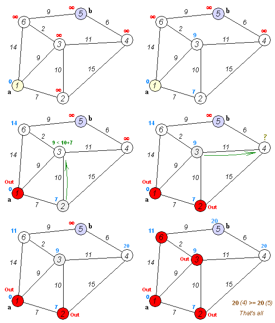
A simulated version of Dijkstra’s algorithm:
Here it is used to find the shortest path between a and b.It picks the unvisited vertex with the lowest distance, calculates the distance through it to each unvisited neighbor, and updates the neighbor's distance if smaller. Mark visited (set to red) when done with neighbors.
Like the Bellman–Ford algorithm, Dijkstra’s algorithm maintains distances to the nodes and reduces them during the search. Dijkstra’s algorithm is efficient, because it only processes each edge in the graph once, using the fact that there
are no negative edges.
Note: This algorithm is very similar to Prim’s algorithm for Minimum Spanning Tree.
Algorithmic steps:
The implementation of Dijkstra’s algorithm calculates the minimum distances from a node s to other nodes of the graph. The graph is stored as adjacency lists so that adj[a] contains a pair (b,w) always when there is an edge
from node a to node b with weight w.
An efficient implementation of Dijkstra’s algorithm requires that it is possible to efficiently find the minimum distance node that has not been processed. An appropriate data structure for this is a priority queue that contains the nodes ordered by their distances. Using a priority queue, the next node to be processed can be retrieved in logarithmic time.( that is, in O(LogN) time complexity).
By default a priority_queue sorts elements in descending order. To make it sort the elements in ascending order, we can either store the negated distances in it, or pass it a different sorting function. We will do the second option.
Implementation:
                                                            const int INF = 1000000000;
vector<vector<pair<int, int>>> adj;

void dijkstra(int s, vector<int> & d, vector<int> & p) {
    int n = adj.size();
    d.assign(n, INF);
    p.assign(n, -1);

    d[s] = 0;
    using pii = pair<int, int>;
    priority_queue<pii, vector<pii>, greater<pii>> q;
    q.push({0, s});
    while (!q.empty()) {
        int v = q.top().second;
        int d_v = q.top().first;
        q.pop();
        if (d_v != d[v])
            continue;

        for (auto edge : adj[v]) {
            int to = edge.first;
            int len = edge.second;

            if (d[v] + len < d[to]) {
                d[to] = d[v] + len;
                p[to] = v;
                q.push({d[to], to});
            }
        }
    }
}
Complexity Analysis:
•Time Complexity: The time complexity of the above implementation is O(E+V*Log(V), because the algorithm goes through all nodes of the graph and adds for each edge at most one distance to the priority queue.
•Space Complexity: O(V+E)
3)Floyd-Warshall Algorithm:
The Floyd–Warshall algorithm provides an alternative way to approach the problem of finding shortest paths. Unlike the other algorithms of this chapter, it finds all shortest paths between the nodes in a single run.
Algorithmic steps:
The key idea of the algorithm is to partition the process of finding the shortest path between any two vertices to several incremental phases.
Let us number the vertices starting from 1 to n. The matrix of distances is d[][].
Initially, the distance of every node from itself is 0. The distance of any node from a node(let's say b) is x-the edge weight if there exists an edge between the two nodes with weight x, else it is initialised to a very large value(we will call it as infinity).
Suppose now that we are in the k-th phase, and we want to compute the matrix d[][] so that it meets the requirements for the (k+1)-th phase. We have to fix the distances for some vertex pairs (i,j). There are two fundamentally different cases:
•The shortest distance from vertex i to vertex j from internal vertices from the set {1,2,3.. K} coincides with the shortest path from internal vertices: {1,2,3..k-1}.
In this case, d[i][j] will not change during the transition.
•The shortest path with internal vertices from {1,2,3,..k} is shorter.
Therefore, it means that the shortest path between i and j is :
d[i][j]=d[i][k]+d[k][j];
Combining the two cases, we can recalculate the length of all pairs (i,j) in the k-th phase in the following way:
d[i][j]= min(d[i][j],d[i][k]+d[k][j]);
So, after the n-th phase, the shortest path between vertices (i,j) is d[i][j], or it is inf - if there does not exist any node between i and j.
Implementation:
                                                            for (int k = 0; k < n; ++k) {
    for (int i = 0; i < n; ++i) {
        for (int j = 0; j < n; ++j) {
            if (d[i][k] < INF && d[k][j] < INF)
                d[i][j] = min(d[i][j], d[i][k] + d[k][j]);
        }
    }
}
Complexity Analysis:
•Time Complexity: O(n3)
The algorithm involves three nested loops, so its complexity is cubic in nature.
•Space Complexity: O(V2)
Since a 2D array of dimensions V x V is used, it requires a space complexity of the order of O(V2).
Problems on Shortest Path Algorithms
Study Material for Shortest Path Algorithms
Shortest Path Algorithms Tutorials & Notes | Algorithms
Dijsktra's algorithm
Floyd–Warshall algorithm
C/C++ Program for Shortest Path in Directed Acyclic Graph
LEVEL-7: SPECIALIST
Disjoint Set Union
Introduction (DSU)
Before studying disjoint set union we need to know what a set is and what is meant by disjoint.
So a set can be defined as a collection of unique elements and two sets are said to be disjoint if there exists no element which is present in both of them or mathematically we can say,
A ∩ B = ɸ, where A and B be two sets containing similar elements.
Disjoint set Union (DSU) is an advanced Data Structure. It stores disjoint sets in the form of a tree where each tree denotes a single set and the root of the tree is used to represent the entire set.
Let us define 4 sets as
A = {2,4,6,8}
B = {5,3}
C = {1,7}
D = {9}
The representation of these sets will look like:
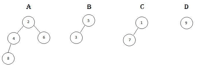
Basic Operations of DSU
A DSU has the following methods. Initially we have several elements and each belong to a unique set. A DSU can
• union_set(u,v) - merge any two sets.
• find_root(x) - tell in which set a specific element is.
• create_set(x) - create a set from a new element.
Thus the three basic operations of DSU are as follows:
• union_set(u, v) - merges the two different sets (the set in which the element u is present and the set in which the element v is present)
In the previous example if we perform union_set(3,7), then B will contain {1,3,5,7} and 1 (or 5) will represent the root of B.
• find_root(x) - returns the root or the element representing the set which contains the element x. We can check if two elements are part of the same set by checking if they have the same root element or not.
if find_root(a) == find_root(b) , then a and b are in the same set, otherwise they are in different sets.
In the previous example, find_root(7) returns 1 and find_root(6) returns 2.
• create_set(x) - creates a new set consisting of the element x.
Implementation of DSU
                                                            void create_set(int x)
{
    dsu[x] = x;
}

int find_root(int x)
{
    if (x == dsu[x])
        return x;
    return find_root(dsu[x]);
}

void union_set(int u, int v)
{
    int a = find_root(u);
    int b = find_root(v);
    if (a != b)
        dsu[b] = a;
}
First let us write all the functions we just read about.
Initially all the elements will represent their own set because there is no set defined. Thus create_set(x) will initialise dsu[x] = x.
Now to find the root of a set we need to check for the parent node’s value. If dsu[x] = x, it means this is the node representing the set or the root node.
To merge two sets we just need to make an edge between the roots of both the sets.
This implementation is quite simple but inefficient. So we will check out how we can optimize these.
Optimization Techniques
Let’s consider the find_root(), the time complexity is O(N) in case of a set represented using a linear tree. If we can change the maximum height of the tree from O(N) to O(log N) just like a balanced tree then the time complexity will also be reduced without affecting the set.
In this example both the trees represent the same set but in the second tree the maximum height is reduced. This optimization technique is known as Path Compression.
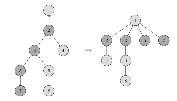
                                                            int find_root(int x)
{
     if (x == dsu[x])
        return x;
     dsu[v] = find_root(dsu[v]);
     return dsu[v];
}
Let’s now check how we can implement this.
In case of Union operation we merge the root of one set with the root of another set. For set A and B having roots x and y respectively, while merging we have two ways:
x will represent the entire set or all the elements in set B will now have x as root.
y will represent the entire set or all the elements in set A will now have y as root.
Which is more optimal?
This depends on the size of the sets. If we merge the smaller set with the bigger then it would be more efficient. So basically we decide which tree will attract the other. To achieve this we will have to keep the size of each set stored in an array.
                                                            int size[n+1];
void create_set(int x)
{
    dsu[x] = x;
    size[x] = 1;
}

void union_set(int u, int v)
{
    int a = find_set(a);
    int b = find_set(b);
    if (a != b)
    {
        if (size[a] < size[b])
            swap(a, b);
        dsu[b] = a;
        size[a] += size[b];
    }
}
Let us now try to implement it.
This implementation is known as Union by Size.
Complete Implementation
                                                        int dsu[n+1];
int size[n+1];

void create_set(int x)
{
    dsu[x] = x;
    size[x] = 1;
}

int find_root(int x)
{
     if (x == dsu[x])
        return x;
     dsu[v] = find_root(dsu[v]);
     return dsu[v];
}

void union_set(int u, int v)
{
    int a = find_set(a);
    int b = find_set(b);
    if (a != b)
    {
        if (size[a] < size[b])
            swap(a, b);
        dsu[b] = a;
        size[a] += size[b];
    }
}

void initialize_dsu(int n)
{
	for(int i=1;i<=n;i++)
		create_set(i);
}
Study Material for DSU
Disjoint-set data structure | Wikipedia
Disjoint Set Union (Union Find) | HackerEarth
Disjoint Set Union | Competitive Programming Algorithms
Tutorials - Disjoint-set Data Structures | Topcoder.com
Segment Tree
Introduction & Operations in Segment Tree
Segment Tree is a basically a binary tree used for storing the intervals or segments. Each node in the Segment Tree represents an interval. Consider an array A of size N and a corresponding Segment Tree T:
1. The root of T will represent the whole array A[0:N−1].
2. Each leaf in the Segment Tree T will represent a single element A[i] such that 0≤i<N.
3. The internal nodes in the Segment Tree T represents the union of elementary intervals A[i:j] where 0≤i<j<N.
The root of the Segment Tree represents the whole array A[0:N−1]. Then it is broken down into two half intervals or segments and the two children of the root in turn represent the A[0:(N−1)/2] and A[(N−1)/2+1:(N−1)]. So in each step, the segment is divided into half and the two children represent those two halves. So the height of the segment tree will be log2N. There are N leaves representing the N elements of the array. The number of internal nodes is N−1. So, a total number of nodes are 2×N−1.
The Segment Tree of array A of size 7 will look like :
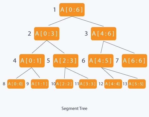
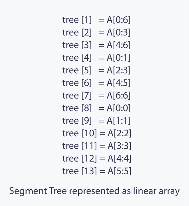
NOTE: Once the Segment Tree is built, its structure cannot be changed. We can update the values of nodes but we cannot change its structure.
Operations in Segment Tree:
1. Update: To update the element of the array A and reflect the corresponding change in the Segment tree.
2. Query: In this operation we can query on an interval or segment and return the answer to the problem (say minimum/maximum/summation in the particular segment).
Implementation of Segment Tree
A Segment Tree can be built using recursion (bottom-up approach ). Start with the leaves and go up to the root and update the corresponding changes in the nodes that are in the path from leaves to root.
For update(), search the leaf that contains the element to update. This can be done by going to either on the left child or the right child depending on the interval which contains the element. Once the leaf is found, it is updated and again use the bottom-up approach to update the corresponding change in the path from that leaf to the root.
To make a query() on the Segment Tree, select a range from L to R (which is usually given in the question). Recurse on the tree starting from the root and check if the interval represented by the node is completely in the range from L to R. If the interval represented by a node is completely in the range from L to R, return that node’s value.
Now, let us look at the code to get a better idea.
                                                            void buildSegTree(vector<int>& arr, int treeIndex, int lo, int hi)
{
    if (lo == hi) {                 // leaf node. store value in node.
        tree[treeIndex] = arr[lo];
        return;
    }

    int mid = lo + (hi - lo) / 2;   // recurse deeper for children.
    buildSegTree(arr, 2 * treeIndex + 1, lo, mid);
    buildSegTree(arr, 2 * treeIndex + 2, mid + 1, hi);

    // merge build results
    tree[treeIndex] = merge(tree[2 * treeIndex + 1], tree[2 * treeIndex + 2]);
}

// call this method as buildSegTree(arr, 0, 0, n-1);
// Here arr[] is input array and n is its size.
Build the tree from the original data.
Complexity of build() is O(N).
                                                            int querySegTree(int treeIndex, int lo, int hi, int i, int j)
{
    // query for arr[i..j]

    if (lo > j || hi < i)               // segment completely outside range
        return 0;                       // represents a null node

    if (i <= lo && j >= hi)             // segment completely inside range
        return tree[treeIndex];

    int mid = lo + (hi - lo) / 2;       // partial overlap of current segment and queried range. Recurse deeper.

    if (i > mid)
        return querySegTree(2 * treeIndex + 2, mid + 1, hi, i, j);
    else if (j <= mid)
        return querySegTree(2 * treeIndex + 1, lo, mid, i, j);

    int leftQuery = querySegTree(2 * treeIndex + 1, lo, mid, i, mid);
    int rightQuery = querySegTree(2 * treeIndex + 2, mid + 1, hi, mid + 1, j);

    // merge query results
    return merge(leftQuery, rightQuery);
}

// call this method as querySegTree(0, 0, n-1, i, j);
// Here [i,j] is the range/interval you are querying.
// This method relies on "null" nodes being equivalent to storing zero.
Read/Query on an interval or segment of the data.
Complexity of query() is O(log N).
                                                            void updateValSegTree(int treeIndex, int lo, int hi, int arrIndex, int val)
{
    if (lo == hi) {                 // leaf node. update element.
        tree[treeIndex] = val;
        return;
    }

    int mid = lo + (hi - lo) / 2;   // recurse deeper for appropriate child

    if (arrIndex > mid)
        updateValSegTree(2 * treeIndex + 2, mid + 1, hi, arrIndex, val);
    else if (arrIndex <= mid)
        updateValSegTree(2 * treeIndex + 1, lo, mid, arrIndex, val);

    // merge updates
    tree[treeIndex] = merge(tree[2 * treeIndex + 1], tree[2 * treeIndex + 2]);
}

// call this method as updateValSegTree(0, 0, n-1, i, val);
// Here you want to update the value at index i with value val.
Update the value of an element.
Complexity of update() is O(log N).
Study Material for Segment Tree
Efficient and easy Segment Trees
Lazy Propagation in Segment Tree
Segment Tree | Competitive Programming Algorithms
Segment Tree | Leetcode Article
LEVEL-8: EXPERT
String Algorithm
String Hashing
Hashing algorithms are helpful in solving a lot of problems.
For the conversion, we need a so-called hash function. The goal of it is to convert a string into an integer, the so-called hash of the string. The following condition has to hold: if two strings s and t are equal (s=t), then also their hashes have to be equal (hash(s)=hash(t)). Otherwise, we will not be able to compare strings.
Notice, the opposite direction doesn't have to hold. If the hashes are equal (hash(s)=hash(t)), then the strings do not necessarily have to be equal.
BRUTE FORCE APPROACH :
We want to solve the problem of comparing strings efficiently. The brute force way of doing so is just to compare the letters of both strings.
● Time Complexity: O(min(n1,n2))
● Space Complexity: S(min(n1,n2))
where n1 and n2 are the sizes of the two strings
OPTIMISED APPROACH :
We want to do better. The idea behind strings is the following: we convert each string into an integer and compare those instead of the strings.
● Time Complexity: O(1)
Rabin Karp
Given a text txt[0..n-1] and a pattern pat[0..m-1], write a function search(char pat[], char txt[]) that prints all occurrences of pat[] in txt[]. You may assume that n > m.
Examples:
Input: txt[] = "THIS IS A TEST TEXT"
pat[] = "TEST"
Output: Pattern found at index 10
Input: txt[] = "AABAACAADAABAABA"
pat[] = "AABA"
Output: Pattern found at index 0
Pattern found at index 9
Pattern found at index 12
The algorithm is as shown :
                                                        function RabinKarp(string s[1..n], string pattern[1..m])
    hpattern := hash(pattern[1..m]);
    for i from 1 to n-m+1
        hs := hash(s[i..i+m-1])
        if hs = hpattern
            if s[i..i+m-1] = pattern[1..m]
                return i
    return not found
Implementation :
                                                        #include <bits/stdc++.h>
using namespace std;

// d is the number of characters in the input alphabet
#define d 256

/* pat -> pattern
    txt -> text
    q -> A prime number
*/
void search(char pat[], char txt[], int q)
{
    int M = strlen(pat);
    int N = strlen(txt);
    int i, j;
    int p = 0; // hash value for pattern
    int t = 0; // hash value for txt
    int h = 1;

    // The value of h would be "pow(d, M-1)%q"
    for (i = 0; i < M - 1; i++)
        h = (h * d) % q;

    // Calculate the hash value of pattern and first
    // window of text
    for (i = 0; i < M; i++)
    {
        p = (d * p + pat[i]) % q;
        t = (d * t + txt[i]) % q;
    }

    // Slide the pattern over text one by one
    for (i = 0; i <= N - M; i++)
    {

        // Check the hash values of current window of text
        // and pattern. If the hash values match then only
        // check for characters on by one
        if ( p == t )
        {
            /* Check for characters one by one */
            for (j = 0; j < M; j++)
            {
                if (txt[i+j] != pat[j])
                    break;
            }

            // if p == t and pat[0...M-1] = txt[i, i+1, ...i+M-1]
            if (j == M)
                cout<<"Pattern found at index "<< i<<endl;
        }

        // Calculate hash value for next window of text: Remove
        // leading digit, add trailing digit
        if ( i < N-M )
        {
            t = (d*(t - txt[i]*h) + txt[i+M])%q;

            // We might get negative value of t, converting it
            // to positive
            if (t < 0)
            t = (t + q);
        }
    }
}

/* Driver code */
int main()
{
    char txt[] = "HELLO, ALL THE BEST";
    char pat[] = "HELLO";

      // A prime number
    int q = 101;

      // Function Call
      search(pat, txt, q);
    return 0;
}

The Average Time Complexity is: O(n-m+1)
Worst Case Complexity is: O(nm)
KMP
The Knuth-Morris-Pratt algorithm is considered one of the best algorithms for solving the pattern matching problem.
The idea behind the algorithm is not too different from the naive string search procedure. As it, Knuth-Morris-Pratt aligns the text with the pattern and goes with character comparisons from left to right. But, instead of making a shift of one character when a mismatch occurs, it uses a more intelligent way to move the pattern along the text. In fact, the algorithm features a pattern pre-processing stage where it acquires all the informations that will make the algorithm skip redundant comparisons, resulting in larger shifts.
The pre-processing stage produces an array (called suffixPrefix in the code) of integers in which every element suffixPrefix[i] records the length of the longest proper suffix of P[0...i] (where P is the pattern) that matches a prefix of P. In other words, suffixPrefix[i] is the longest proper substring of P that ends at position i and that is a prefix of P. Just a quick example. Consider P = "abadfryaabsabadffg", then suffixPrefix[4] = 0, suffixPrefix[9] = 2, suffixPrefix[14] = 4.
WORKING :
Once the shift-array suffixPrefix is ready we can begin with pattern search stage. The algorithm first attempts to compare the characters of the text with those of the pattern. If it succeeds, it goes on until a mismatch occurs. When it happens, it checks if an occurrence of the pattern is present (and reports it). Otherwise, if no comparisons are made then the text cursor is moved forward, else the pattern is shifted to the right. The shift's amount is based on the suffixPrefix array, and it guarantees that the prefix P[0...suffixPrefix[i]] will match its opposing substring in the text. In this way, shifts of more than one character are often made and lot of comparisons can be avoided, saving a lot of time.
Let's make an example reasoning with the code above. Let's consider the string P = ACTGACTA", the consequentially obtained suffixPrefix array equal to [0, 0, 0, 0, 0, 0, 3, 1], and the text T = "GCACTGACTGACTGACTAG". The algorithm begins with the text and the pattern aligned like below. We have to compare T[0] with P[0].

We have a mismatch and we move on comparing T[1] and P[0]. We have to check if a pattern occurrence is present but there is not. So, we have to shift the pattern right and by doing so we have to check suffixPrefix[1 - 1]. Its value is 0 and we restart by comparing T[1] with P[0]. Again a mismath occurs, so we go on with T[2] and P[0].
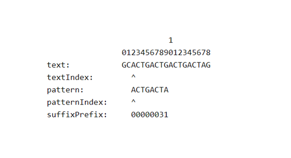
This time we have a match. And it continues until position 8. Unfortunately the length of the match is not equal to the pattern length, we cannot report an occurrence. But we are still lucky because we can use the values computed in the suffixPrefix array now. In fact, the length of the match is 7, and if we look at the element suffixPrefix[7 - 1] we discover that is 3. This information tell us that that the prefix of P matches the suffix of the susbtring T[0...8]. So the suffixPrefix array guarantees us that the two substring match and that we do not have to compare their characters, so we can shift right the pattern for more than one character!
The comparisons restart from T[9] and P[3].
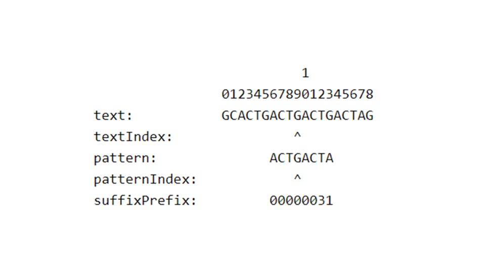
They match so we continue the compares until position 13 where a misatch occurs beetwen charcter G and A.
Just like before, we are lucky and we can use the suffixPrefix array to shift right the pattern.

Again, we have to compare. But this time the comparisons finally take us to an occurrence, at position 17 - 7 = 10.
The algorithm than tries to compare T[18] with P[1] (because we used the element suffixPrefix[8 - 1] = 1) but it fails and at the next iteration it ends its work.
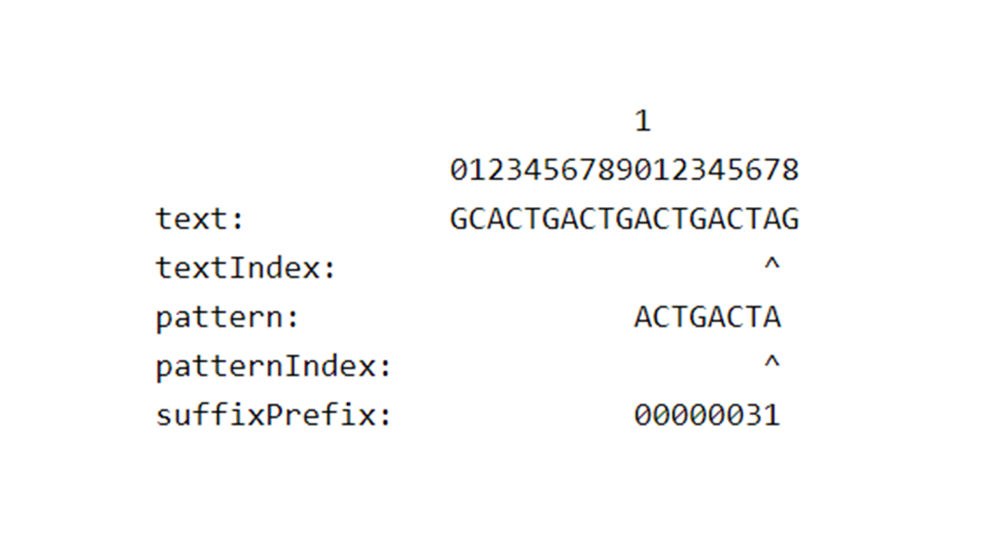
The pre-processing stage involves only the pattern. The running time of the Z-Algorithm is linear and takes O(n), where n is the length of the pattern P. After that, the search stage does not "overshoot" the length of the text T (call it m). It can be be proved that number of comparisons of the search stage is bounded by 2 * m. The final running time of the Knuth-Morris-Pratt algorithm is O(n + m).
                                                        void preKMP(string pattern, int f[])
{
    int m = pattern.length(), k;
    f[0] = -1;
    for (int i = 1; i < m; i++)
    {
        k = f[i - 1];
        while (k >= 0)
        {
            if (pattern[k] == pattern[i - 1])
                break;
            else
                k = f[k];
        }
        f[i] = k + 1;
    }
}

//check whether target string contains pattern
bool KMP(string pattern, string target)
{
    int m = pattern.length();
    int n = target.length();
    int f[m];
    preKMP(pattern, f);
    int i = 0;
    int k = 0;
    while (i < n)
    {
        if (k == -1)
        {
            i++;
            k = 0;
        }
        else if (target[i] == pattern[k])
        {
            i++;
            k++;
            if (k == m)
                return 1;
        }
        else
            k = f[k];
    }
    return 0;
}
Useful Links KMP
Z Algorithm
Z-Algorithm is foremost an algorithm that process a pattern in order to calculate a skip-comparisons-table.
The computation of the Z-Algorithm over a pattern P produces an array (called Z) of integers in which each element, call it Z[i], represents the length of the longest substring of P that starts at i and matches a prefix of P. In simpler words, Z[i] records the longest prefix of P[i...|P|] that matches a prefix of P. As an example, let's consider P = "ffgtrhghhffgtggfredg". We have that Z[5] = 0 (f...h...), Z[9] = 4 (ffgtr...ffgtg...) and Z[15] = 1 (ff...fr...).
But how do we compute Z? Before we describe the algorithm we must introduce the concept of Z-box. A Z-box is a pair (left, right) used during the computation that records the substring of maximal length that occurs also as a prefix of P. The two indices left and right represent, respectively, the left-end index and the right-end index of this substring.
The definition of the Z-Algorithm is inductive and it computes the elements of the array for every position k in the pattern, starting from k = 1. The following values (Z[k + 1], Z[k + 2], ...) are computed after Z[k]. The idea behind the algorithm is that previously computed values can speed up the calculus of Z[k + 1], avoiding some character comparisons that were already done before.
Let's make an example reasoning with the code above. Let's consider the string P = “abababbb". The algorithm begins with k = 1, left = right = 0. So, no Z-box is "active" and thus, because k > right we start with the character comparisons between P[1] and P[0].
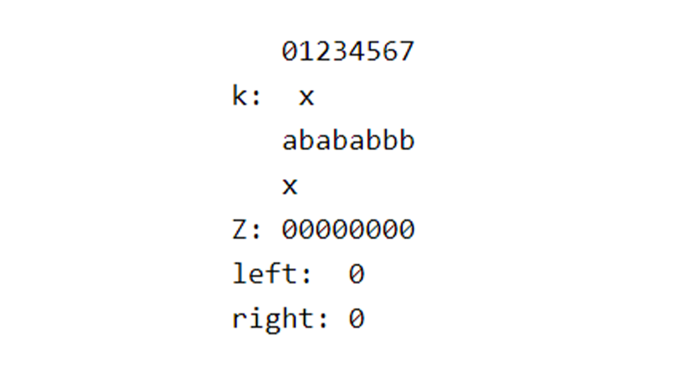
We have a mismatch at the first comparison and so the substring starting at P[1] does not match a prefix of P. So, we put Z[1] = 0 and let left and right untouched. We begin another iteration with k = 2, we have 2 > 0 and again we start comparing characters P[2] with P[0]. This time the characters match and so we continue the comparisons until a mismatch occurs. It happens at position 6. The characters matched are 4, so we put Z[2] = 4 and set left = k = 2 and right = k + Z[k] - 1 = 5. We have our first Z-box that is the substring "abab" (notice that it matches a prefix of P) starting at position left = 2.
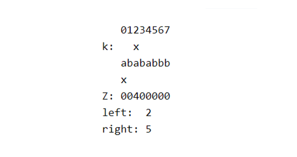
We then proceed with k = 3. We have 3 <= 5. We are inside the Z-box previously found and inside a prefix of P. So we can look for a position that has a previously computed value. We calculate k_1 = k - left = 1 that is the index of the prefix's character equal to P[k]. We check Z[1] = 0 and 0 < (right - k + 1 = 3) and we find that we are exactly inside the Z-box. We can use the previously computed value, so we put Z[3] = Z[1] = 0, left and right remain unchanged.
At iteration k = 4 we initially execute the else branch of the outer if. Then in the inner if we have that k_1 = 2 and (Z[2] = 4) >= 5 - 4 + 1. So, the substring P[k...r] matches for right - k + 1 = 2 chars the prefix of P but it could not for the following characters. We must then compare the characters starting at r + 1 = 6 with those starting at right - k + 1 = 2. We have P[6] != P[2] and so we have to set Z[k] = 6 - 4 = 2, left = 4 and right = 5.
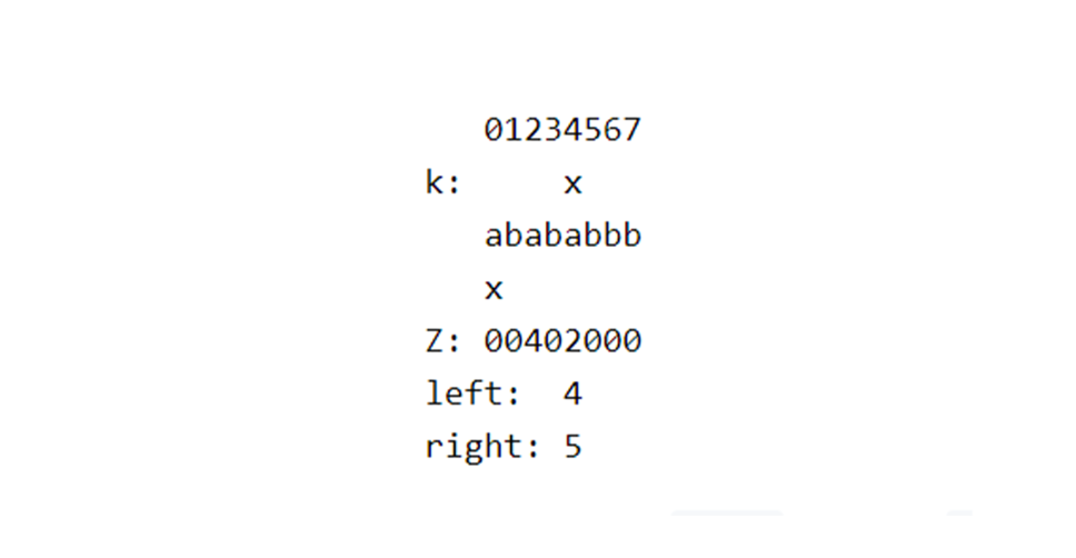
With iteration k = 5 we have k <= right and then (Z[k_1] = 0) < (right - k + 1 = 1) and so we set z[k] = 0. In iteration 6 and 7 we execute the first branch of the outer if but we only have mismatches, so the algorithms terminates returning the Z-array as Z = [0, 0, 4, 0, 2, 0, 0, 0].
The Z-Algorithm runs in linear time. More specifically, the Z-Algorithm for a string P of size n has a running time of O(n).
                                                        bool zAlgorithm(string pattern, string target)
{
    string s = pattern + '$' + target;
    int n = s.length();
    vector<int> z(n, 0);
    int goal = pattern.length();
    int r = 0, l = 0, i;
    for (int k = 1;  k < n; k++)
    {
        if (k > r)
        {
            for (i = k; i < n && s[i] == s[i - k]; i++);
            if (i > k)
            {
                z[k] = i - k;
                l = k;
                r = i - 1;
            }
        }
        else
        {
            int kt = k - l, b = r - k + 1;
            if (z[kt] > b)
            {
                for (i = r + 1; i < n && s[i] == s[i - k]; i++);
                z[k] = i - k;
                l = k;
                r = i - 1;
            }
        }
        if (z[k] == goal)
            return true;
    }
    return false;
}
Useful Links Z-Algorithm
LEVEL-9: MASTER
Dynamic Programming
Introduction (DP)
Dynamic programming is a method for solving a complex problem by breaking it down into a collection of simpler subproblems.
Dynamic programming (referred as DP from now) is a process where you will store the data (or solutions) which are solved previously and use them in further calculations.
Example:
if you are asked to calculate a product of the first 5 numbers then you calculated it and it turns out to be 120 . Now you are asked to calculate the product of the first 6 numbers.
Do you again calculate as 1*2*3*4*5*6
Or smartly calculate 120*6
Give this smartness to your code and integrating this to your code is the concept of DP
                                                            int fib (int n) {
   // Base Case
   if (n < 2)
       return 1;
   return fib(n-1) + fib(n-2);
}
The concept of DP came into picture due to the overlapping subproblems. Taking fibonacci numbers as example lets see about overlapping sub problems.
Now lets try to calculate fib[6]
Clearly we can see fib(4) is calculating 2 times and fib(3) is calculating thrice.
So a particular subproblem is calculating more than once resulting in time waste.
For eliminating this we want to memorize the previous answers.
Lets see different ways to do this.
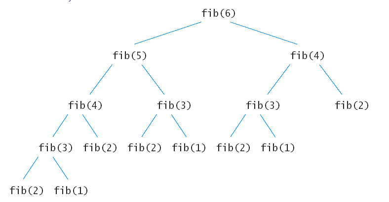
What are States of DP?
● State represents the Data unit required for further calculation
● For a particular state there exists only one solution
Example : Considering The previous example fib(5) is a state fib(4) is a state
Example : suppose you are dealing with sub arrays in a array so you require at least 2 variables to specify a particular sub array
● startIndex,endIndex
● (or)startIndex,length
● Or any other convention you follow
Suppose you are involved in a DP problem which requires dealing with sub arrays then at least these 2 variables are needed for further calculation and these two combinedly called as a state.
Reference problems : LCS and LIS
Different Approaches in DP
BOTTOM UP :
                                                            int main()
{
   int n=10;
   int fibArr[n];
   fibArr[0]=fibArr[1]=1;
   for(int i=2;i<n;i++)
     {
         fibArr[i]=fibArr[i-1]+fibArr[i-2];
     }
}
We try to calculate the bottom values and use it for further calculation. I.e if we take an example of fibonacci numbers we start from base cases fib(0),fib(1) and calculate fib(2) then fib(3) then fib(4) etc…
● For storing the answers we can use a array and fill it using a loop
● As this is like preparing a table sometimes this approach is also referred as Tabulation
In tabulation we will calculate all values upto a particular value (n) which is required
TOP DOWN :
                                                            int fibArr[100001];
int fib(int n){
   if(fibArr[n]!=0)
     {
          fibArr[n]=fib(n-1)+fib(n-2);
      }
   return fibArr[n];
}
int main()
{
   fill(fibArr,fibArr+100001,0);
   fibArr[0]=fibArr[1]=1;
   cout<<fib(10);
}
We try to calculate the top value which requires a bottom one so we will calculate it
● We can use recursion concept and uses a global (or passed to function) array
● This approach is also referred to as Memorization
While using a top-down approach we will calculate a particular value only when it is needed. This will save a lot of time depending upon the problem.
Example: let's consider this
● F(n)=F(n/2)+1 (where n/2 represents integer division)
● With base F(0)=1
To calculate F(1024) bottom-up(iterative approach) takes 1024 steps whereas top-down approach takes only 10 steps.
RECURSIVE AND ITERATIVE APPROACHES :
● Generally iterative approaches are better than recursive approaches from a compiler(computer’s) perspective.
● But Recursive approach is easy to write in many cases.
● In general bottom-up approach (tabulation) is iterative and top-down approach uses recursive approach.
● But a piece of code which is written recursively can also be written in iterative approach and vice versa.
SAFE CHECKING :
● Recursion uses stack while processing.
● Each language has a particular depth limit in recursion which is the size of stack. It is also referred to as safe checking limit as it ensures that the system won't crash in case of mistakes.
● Generally this is very high in C++ but languages like python and java has low limits compared to C++
● To solve this in python we can add two lines

● Check about handling this over internet for the language which you use.
Examples
1.STAIRCASE PROBLEM :
Problem :
You are climbing a stair case and it takes A steps to reach to the top.
Each time you can either climb 1 or 2 steps. In how many distinct ways can you climb to the top?
Approach :
we can step either 1 step or 2 steps So just make a move and call recursively
If one step decrease step count by 1 similarly do for 2 steps
                                                            //Assuming to call from main function
int Solution::climbStairs(int A) {
    if(A==0)return 1;
    if(A<0)return 0;
    return climbStairs(A-1)+climbStairs(A-2);
}
// This will give tle
We can prove very easily that there are many overlapping subproblems .
Example :
With A small case of A=10 and a small expansion, we end up with two similar states A=8 and two similar states A=7
And this is very large in the case of large values of A.
So we can add the concept of DP to this problem.
This time we use a tabular method for DP by filling the base cases.
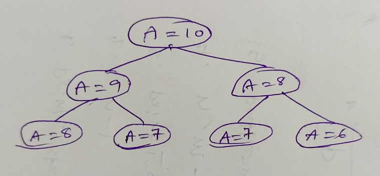
                                                        int Solution::climbStairs(int A) {
    // base case return without filling in array
        if(A==1)return 1;
        if(A==2)return 2;
        int DP[A+1];
    // base cases
        DP[1]=1;
        DP[2]=2;// direct 2 steps or 1+1
        for(int i=3;i<=A;i++){
    // core logic
        DP[i]=DP[i-1]+DP[i-2];
    }
    return DP[A];
}
2. SUBSET SUM :
Problem :
Given an integer array A of size N.
You are also given an integer B, you need to find whether their exist a subset in A whose sum equal B.
If there exists a subset then return 1 else return 0.
Approach :
Selecting a set is very simple. We can either select a particular element or drop a particular element. Here our theme is to find if sum = B or not. So let's think recursively .
Let's consider the last element then we can either consider it or not.
If we considered it then we subtract its value from required sum and proceed to rest n-1 elements else we proceed to rest n-1 elements without modifying
                                                            //Assuming solve function is called from main
bool isPosible(vector<int> &A, int B,int n){
    if(B==0)return true;
    if(B<0||n==0)return false;
    if(isPosible(A,B,n-1)||isPosible(A,B-A[n-1],n-1)){
        return true;
    }
    return false;
}
int solve(vector<int> &A, int B) {
    return isPosible(A,B,A.size())?1:0;
}
This solution will give you TLE for good testcases. You can observe some cases manually and find that overlapping subproblem. So, introduce the concept of DP.
Here we can use 2d dp with one dimension as B. I am using unordered_map. We can use anything for DP. Try the same problem with vectors too.
                                                        //assuming solve function is called from main
bool isPosible(vector<int> &A, int B,int n,unordered_map <int,bool> *dp){
    if(B==0)return true;
    if(B<0||n==0)return false;
    if(dp[B].find(n)!=dp[B].end())
        return dp[B][n];
    return dp[B][n]=(
        isPosible(A,B,n-1,dp)||
        isPosible(A,B-A[n-1],n-1,dp)
    );
}
int Solution::solve(vector<int> &A, int B) {
    unordered_map <int,bool> dp[B+1];
    return isPosible(A,B,A.size(),dp)?1:0;
}
3. COIN CHANGE :
Problem :
Given a value N your required amount to buy something, find the number of ways to make change for N rupees, if we have infinite supply of each of S = { S1, S2, .. , SM } valued coins.
Recursive solution :
In general we can either consider the last coin in our count or we can ignore the last coin which results in recursive calling twice from our code
● If we didnt consider last coin then reduce vlue of m by 1 and again call the function
● Else consider the last coin once and decrease the value of n as per value of the coin .
                                                            long long int count( int S[], int m, int n ){
        if(n==0)return 1;
        if(n<0||m<1)return 0;
        return count(S,m-1,n)+count(S,m,n-S[m-1]);
}
But this approach results in TLE for good test cases.
We can conclude that we are calculating some values multiple times
Lets consider s={3,2,1} means m=3
Ans we need to calculate for n=10
Now we can call count(s,3,10) and it will proceed like this.
In this small expansion (s,2,8) appeared twice.
Similarly on large values, there are many possible overlaps
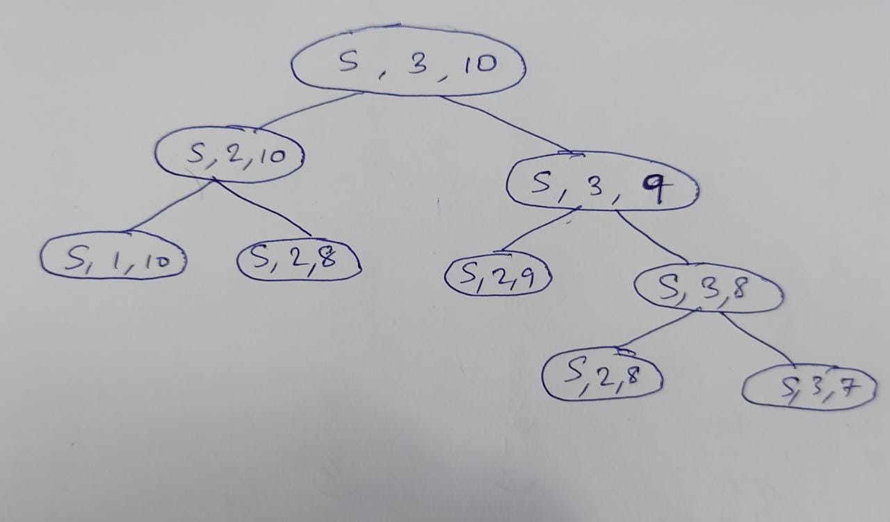
DP Solution :
So due to the overlapping nature of states we use DP
Apply a 2d dp DP[m][n] which corresponds to possible answer of state (s,m,n)
Solution
                                                        // count is called from main
long long int countDP( int S[], int m, int n,map<pair<int,int>,long long int> &DP )
    {
        if(n==0)return 1;
        if(n<0||m<1)return 0;
        // check if its currently in map or not
        if(DP.find({m,n})==DP.end())
            return DP[{m,n}]=countDP(S,m-1,n,DP)+countDP(S,m,n-S[m-1],DP);
        else return DP[{m,n}];
    }
    long long int count(int S[],int m,int n){
        map <pair<int,int>,long long int> DP;
        return count2(S,m,n,DP);
    }
I used a map here just to state that we no need to stick on vectors or arrays but also use any other thing if you feel it is suitable. You try the same problem to solve with a vector or an array.
And also map takes more time than array So my code probably results to tle sometimes
Useful Links DP
LongestPalindromicSubstring
LongestPalindromicSubsequence
MinSumPathInMatrix
ProblemSet : Interview Bit
LCS
Problem Statement : Given two sequences, find the length of longest subsequence present in both of them.
Note : A subsequence is a sequence that appears in the same relative order, but not necessarily contiguous. For example, “abc”, “abg”, “bdf”, “aeg”, ‘”acefg”, .. etc are subsequences of “abcdefg”
LCS example
String 1 : ABQZGH
String 2 : AEZPHR
LCS : AZH
Approach
The naive solution which includes generating all subsequences of both given sequences and finding the longest matching subsequence. But, this solution takes up exponential time.
Let’s observe some things,
Take s1 of length m and s2 of length n.
i) If last characters, that is, s1[m-1] and s2[n-1] matches then,
LCS(s1[0..m-1],s2[0...n-1]) = 1 + LCS(s1[0..m-2],s2[0...n-2])
ii) If last characters, that is, s1[m-1] and s2[n-1] do not match then,
LCS(s1[0..m-1],s2[0...n-1])
= Maximum( LCS(s1[0..m-1],s2[0...n-2]),LCS(s1[0..m-2],s2[0...n-1])
Therefore, it has optimal substructure.
It can be solved using Recursion.
Let’s implement this by taking s1=”AXYT” and s2=”AYZX”
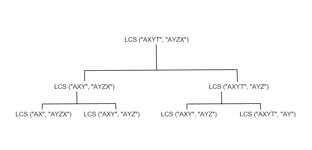
So, we see LCS(“AXY”,”AYZ”) being called twice if we only use recursion. Similarly, if we draw the tree further, we find that it has many overlapping substructures.
Hence, as this problem has both an optimal and overlapping substructure property, it can be seen as a Dynamic Programming Problem.
Solution Using Memoization :
                                                        int LCS(string X, string Y, int m, int n)
{
    // base condition
    if (m == 0 || n == 0)
        return 0;
    // to avoid recomputation of same subproblem
    if (dp[m - 1][n - 1] != -1)
        return dp[m - 1][n - 1];
    if (X[m - 1] == Y[n - 1]) {
        // store it in dp array to avoid recomputation in future
        dp[m - 1][n - 1] = 1 + lcs(X, Y, m - 1, n - 1, dp);
        return dp[m - 1][n - 1];
    }
    else {
        // store it in dp array to avoid recomputation in future
        dp[m - 1][n - 1] = max(lcs(X, Y, m, n - 1, dp),
                               lcs(X, Y, m - 1, n, dp));
        return dp[m - 1][n - 1];
    }
}
Solution Using Tabulation :
                                                        int LCS( string X, string Y, int m, int n )
{
    int dp[m + 1][n + 1];
    int i, j;

    /*Note that L[i][j] contains length of LCS of X[0..i-1] and Y[0..j-1] */
    for (i = 0; i <= m; i++)
    {
        for (j = 0; j <= n; j++)
        {
        if (i == 0 || j == 0)
            dp[i][j] = 0;

        else if (X[i - 1] == Y[j - 1])
            dp[i][j] = dp[i - 1][j - 1] + 1;

        else
            dp[i][j] = max(dp[i - 1][j], dp[i][j - 1]);
        }
    }

    /* L[m][n] contains length of LCS for X[0..n-1] and Y[0..m-1] */
    return L[m][n];
}
Problems which are variations of LCS
LIS
The Longest Increasing Subsequence (LIS) problem is to find the length of the longest subsequence of the given sequence such that all elements of the subsequence are sorted in increasing order.
LIS example:
Arr : {11, 25, 9, 34, 21, 51, 41, 70, 91}
LIS length : 6 ( LIS is {11, 25, 34, 51, 70, 91} )
Approach :
Let LIS(i) be the length of the LIS ending at index i such that arr[i] is the last element of the LIS.
Then, these are the two cases possible,
i) LIS(i) = 1 + max( LIS(j) ) where 0 < j < i and arr[j] < arr[i]
ii) LIS(i) = 1, if no such j exists.
Thus, we see the LIS problem satisfies the optimal substructure property as the optimal solution can be reached using solutions to subproblems.
Hence, can be solved by Recursion.
Lets see an example
Input : arr[] = {5, 12, 4, 13}
LIS(1)=1
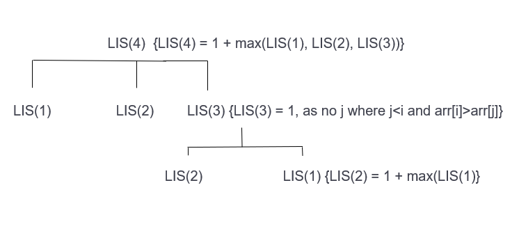
So, we can see overlapping substructures.
Solution Using Tabulation :
                                                        int LIS( int arr[], int n )
{
    int lis[n];
    lis[0] = 1;
    for (int i = 1; i < n; i++ )
    {
        lis[i] = 1;
        for (int j = 0; j < i; j++ )
            if ( arr[i] > arr[j] && lis[i] < lis[j] + 1)
                lis[i] = lis[j] + 1;
    }
    int ans=0;
    for(int i=0;i<n;i++)
	ans=max(ans,lis[i]);

    // Return maximum value in lis[]
    return ans;
}
                                                            //Implementation
int lis(vector<int> const& a) {
    int n = a.size();
    const int INF = 1e9;
    vector<int> lis(n+1, INF);
    lis[0] = -INF;
    for (int i = 0; i < n; i++) {
        for (int j = 1; j <= n; j++) {
            if (lis[j-1] < a[i] && a[i] < lis[j])
                lis[j] = a[i];
        }
    }

    int ans = 0;
    for (int i = 0; i <= n; i++) {
        if (lis[i] < INF)
            ans = i;
    }
    return ans;
}
Optimisation by using DP with binary search
In order to do this, we first make a solution different from previous code using only dp. The change would be that lis(i) in this solution would be denoting the element at which a subsequence of length i terminates. If there are multiple such sequences, then we take the one that ends in the smallest element.
One thing to note is that The array lis will always be sorted: lis[i−1]≤lis[i] for all i=1…n. And also the element a[i] will only update at most one value lis[j].
Thus we can find this element in the array lis[] using binary search in O(log(n))
                                                        //Implementation
int lis(vector<int> const& a) {
    int n = a.size();
    const int INF = 1e9;
    vector<int> lis(n+1, INF);
    lis[0] = -INF;

    for (int i = 0; i < n; i++) {
        int j = upper_bound(lis.begin(), lis.end(), a[i]) - lis.begin();
        if (lis[j-1] < a[i] && a[i] < lis[j])
            lis[j] = a[i];
    }

    int ans = 0;
    for (int i = 0; i <= n; i++) {
        if (lis[i] < INF)
            ans = i;
    }
    return ans;
}
Study Material for LIS
LEVEL-10: PROFESSIONAL
Advanced
Mo's algorithm
Let's take up an example to better understand MO’s Algorithm,
Problem :
Given an array of size N. (Ai <= N)
Answer M number of queries, in each find the count of numbers whose frequency >= 3 in [L,R].
Naive Solution :
Traverse each query one by one, keep the count of each number encountered in that query in an array say count[], traverse count[], check if count[i]>=3, increment “answer” if yes.
Time Complexity = O (N*M)
Slightly Improved Solution :
Initially we looped from L to R, but now we will change the positions from previous query to adjust to current query.
If the previous query was L=3, R=10, then we will have currentL=3 and currentR=10 by the end of that query. Now if the next query is L=5, R=7, then we move the currentL to 5 and currentR to 7.
“add function” means we are adding the element at position to our current set and updating the answer accordingly.
“remove function” means we are deleting the element at position from our current set and updating the answer accordingly.
add(position):
count[array[position]]++
if count[array[position]] == 3:
answer++
remove(position):
count[array[position]]--
if count[array[position]] == 2:
answer--
currentL = 0
currentR = 0
answer = 0
count[] = 0
for each query:
// currentL should go to L, currentR should go to R
while currentL &lt; L:
remove(currentL)
currentL++
while currentL &gt; L:
add(currentL)
currentL--
while currentR &lt; R:
add(currentR)
currentR++
while currentR &gt; R:
remove(currentR)
currentR--
output answer
Solving the above question using MO’s algorithm :
MO’s algorithm is just an order in which we process the queries. We were given M queries, we will re-order the queries in a particular order and then process them. Clearly, this is an offline algorithm. Each query has L and R, we will call them opening and closing. Let us divide the given input array into Sqrt(N) blocks. Each block will be N / Sqrt(N) = Sqrt(N) size. Each opening has to fall in one of these blocks. Each closing has to fall in one of these blocks.
A query belongs to the P'th block if the opening of that query falls in the P'th block. In this algorithm we will process the queries of the 1st block. Then we process the queries of the 2nd block and so on.. finally Sqrt(N)’th block. We already have an ordering, queries are ordered in the ascending order of its block. There can be many queries that belong to the same block.
From now, I will ignore all the blocks and only focus on how we query and answer block 1. We will similarly do for all blocks. All of these queries have their opening in block 1, but their closing can be in any block including block 1. Now let us reorder these queries in ascending order of their R value. We do this for all the blocks.
What does the final order look like?
All the queries are first ordered in ascending order of their block number (block number is the block in which its opening falls). Ties are ordered in ascending order of their R value.
For example consider following queries and assume we have 3 blocks each of size 3.
{0, 3} {1, 7} {2, 8} {7, 8} {4, 8} {4, 4} {1, 2}
Let us re-order them based on their block number.
{0, 3} {1, 7} {2, 8} {1, 2} {4, 8} {4, 4} {7, 8}
Now let us re-order ties based on their R value.
{1, 2} {0, 3} {1, 7} {2, 8} {4, 4} {4, 8} {7, 8}
Now we use the same code stated in the previous section and solve the problem. Above algorithm is correct as we did not do any changes but just reordered the queries.
Proof for complexity of above algorithm – O(Sqrt(N) * N) :
We are done with MO’s algorithm, it is just an ordering. Awesome part is its runtime analysis. It turns out that the O(N^2) code we wrote works in O(Sqrt(N) * N) time if we follow the order specified above. Thats awesome right, with just reordering the queries we reduced the complexity from O(N^2) to O(Sqrt(N) * N), and that too without any further modification to code. Hurray! we will get AC with O(Sqrt(N) * N).
Have a look at our code above, the complexity over all queries is determined by the 4 while loops. First 2 while loops can be stated as “Amount moved by left pointer in total”, second 2 while loops can be stated as “Amount moved by right pointer”. Sum of these two will be the overall complexity.
Most important. Let us talk about the right pointer first. For each block, the queries are sorted in increasing order, so clearly the right pointer (currentR) moves in increasing order. During the start of the next block the pointer possibly at the extreme end will move to least R in the next block. That means for a given block, the amount moved by the right pointer is O(N). We have O(Sqrt(N)) blocks, so the total is O(N * Sqrt(N)). Great!
Let us see how the left pointer moves. For each block, the left pointer of all the queries fall in the same block, as we move from query to query the left pointer might move but as previous L and current L fall in the same block, the moment is O(Sqrt(N)) (Size of the block). In each block the amount left pointer movies is O(Q * Sqrt(N)) where Q is the number of queries falling in that block. Total complexity is O(M * Sqrt(N)) for all blocks.
There you go, total complexity is O( (N + M) * Sqrt(N)) = O( N * Sqrt(N))
When and Where to use this algorithm :
As mentioned, this algorithm is offline, that means we cannot use it when we are forced to stick to given order of queries. That also means we cannot use this when there are update operations. Not just that, there is one important possible limitation: We should be able to write the functions add and remove. There will be many cases where add is trivial but remove is not. One such example is where we want maximum in a range. As we add elements, we can keep track of maximum. But when we remove elements it is not trivial. Anyways in that case we can use a set to add elements, remove elements and report minimum. In that case the add and delete operations are O(log N) (Resulting in O(N * Sqrt(N) * log N) algorithm).
There are many cases where we can use this algorithm. In a few cases we can also use other Data Structures like segment trees, but for a few problems using MO’s algorithm is a must.
Other Related Topics :
1. Square-Root (SQRT) Decomposition
2. MO’s algorithm on Trees
Study Material for Mo's Algorithm
HLD
Balanced Binary Tree
A balanced binary tree, also referred to as a height-balanced binary tree, is defined as a binary tree in which the height of the left and right subtree of any node differ by not more than 1.
Unbalanced Binary Tree
Binary tree in which the height of the left and right subtree of at least one node is more than 1.
Why is an Unbalanced Tree bad?
Height of an unbalanced tree can be arbitrary. In the worst case, we have to visit O(N) nodes to move from one node to another node. So unbalanced trees are not computation friendly.
Consider this Example:
Suppose we have an unbalanced weighted tree(not necessarily a Binary Tree) of n nodes and we have to perform q operations, each can be of one of the two types:
change(a,b): Update weight of the ath edge to b
SumEdge(a,b): Print the sum of edge weight on the path from node a to node b.
Simple Solution:
A Simple solution is to traverse the complete tree for any query. Time complexity of every query in this solution is O(n).
Optimised Solution:
Prerequisites - Segment Tree, Least Common Ancestor
When we look closely at this image we find out that if we break the tree where we have more than one child then we will be left with several linear structures and we know an algorithm for similar queries on linear structure “Segment Tree”.

Here are the details after the trick
The tree still has N nodes, but it is DECOMPOSED into 3 chains each of size N/3. See 3 different colors, each one is a chain.
A and D belong to the same chain. We can get the required sum of node values of path from A to D in O( log N ) time using segment tree data structure.
B belongs to the yellow chain, and D belongs to the blue chain. Path from B to D can be broken as B to T3 and T4 to D. Now we are dealing with 2 cases which are similar to the above case. We can calculate the required sum in O( log N ) time for B to T3 and O( log N ) time for T4 to D. Great, we reduced this to O( log N ).
C belongs to the red chain, and D belongs to the blue chain. Path from C to D can be broken as C to T1, T2 to T3 and T4 to D. Again we are dealing with 3 cases similar to the 2nd case. So we can again do it in O( log N ).
Here, we observe that in the given example only 2 nodes had degrees greater than 2. We did simple decomposition and achieved the solution but as we all know trees are more complex than that, so we need something more to achieve better complexity. This can be done with the help of Heavy Light Decomposition
Approach:
We will divide the tree into several chains such that no two chains have a node in common.
Let us assume we have to find sum from any node X to node Y. Clearly, if the path from X to Y is not broken then we will have a single linear structure and can be easily done by segment tree. Now if the path is broken then we will break the path into two paths- X to LCA(X,Y) and Y to LCA(X,Y) [LCA means least common ancestor]. So our solution will be sum of both the paths
Implementation:
                                                        void HLD(int curNode, int cost, int prev) {
    if(chainHead[chainNo] == -1) {
        chainHead[chainNo] = curNode; // Assign chain head
    }
    chainInd[curNode] = chainNo;
    posInBase[curNode] = ptr; // Position of this node in baseArray which we will use in Segtree
    baseArray[ptr++] = cost;

    int sc = -1, ncost;
    // Loop to find special child
    for(int i=0; i<adj[curNode].size(); i++) if(adj[curNode][i] != prev) {
        if(sc == -1 || subsize[sc] < subsize[adj[curNode][i]]) {
            sc = adj[curNode][i];
            ncost = costs[curNode][i];
        }
    }

    if(sc != -1) {
        // Expand the chain
        HLD(sc, ncost, curNode);
    }

    for(int i=0; i<adj[curNode].size(); i++) if(adj[curNode][i] != prev) {
        if(sc != adj[curNode][i]) {
            // New chains at each normal node
            chainNo++;
            HLD(adj[curNode][i], costs[curNode][i], curNode);
        }
    }
}
Study Material for HLD
Geometric Algorithms
Graham Scan Algorithm
Graham's Scan Algorithm is an efficient algorithm for finding the convex hull of a finite set of points in the plane with time complexity O(N log N). The algorithm finds all vertices of the convex hull ordered along its boundary. It uses a stack to detect and remove concavities in the boundary efficiently.
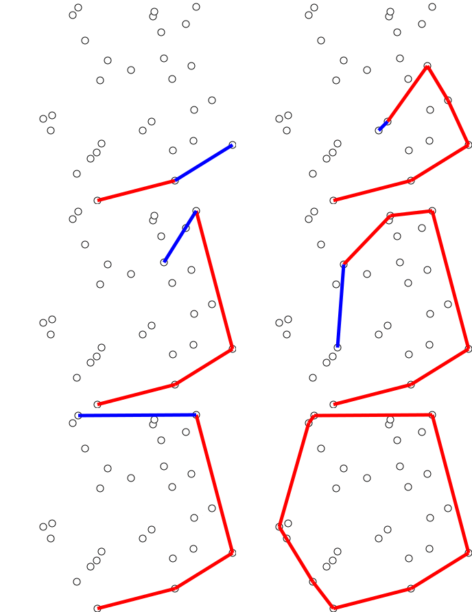
WORKING :
There exist many algorithms that exhibit a better worst-case runtime than Jarvis’ Wrap.
Here we discuss only one of them: a particularly elegant and easy-to-implement variant of the so called Graham Scan [5]. This algorithm is referred to as Successive Local Repair because it starts with some polygon enclosing all points and then step-by-step repairs the deficiencies of this polygon, by removing non-convex vertices. It goes as follows:
Sort points lexicographically and remove duplicates: (p1, . . . , pn).
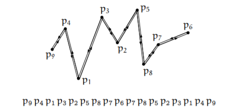
As long as there is a (consecutive) triple (p, q, r) such that r is to the right of or on the
directed line pq, remove q from the sequence.
PSEUDOCODE :
The Pseudocode of Graham Scan Algorithm is as follows:
                                                        let N = number of points
let points[N+1] = the array of points
swap points[1] with the point with the lowest y-coordinate
sort points by polar angle with points[1]
    # We want points[0] to be a sentinel point that will stop the loop.
let points[0] = points[N]
    # M will denote the number of points on the convex hull.
let M = 1
for i = 2 to N:
    # Find next valid point on convex hull.
    while ccw(points[M-1], points[M], points[i]) <= 0:
        if M > 1:
            M -= 1
            continue
        # All points are collinear
        else if i == N:
            break
        else
            i += 1
    # Update M and swap points[i] to the correct place.
    # This code is wrong as explained in the talk page. When M and i are the same,
    the algorithm ends up in an infinite loop.
M += 1
swap points[M] with points[i]
IMPLEMENTATIONS :
Following is the implementation of Graham Scan Algorithm in C++:
                                                        using namespace std;
typedef long long lld;

struct Point
{
    double X, Y;
    Point()
    {
        this->X = this->Y = 0;
    }
    Point(double x, double y)
    {
        this->X = x;
        this->Y = y;
    }
};

int n;
Point P[MAX_N];
Point R;

inline bool cmp(Point A, Point B)
{
    return atan2(A.Y-R.Y,A.X-R.X) < atan2(B.Y-R.Y,B.X-R.X);
}

inline double CCW(Point a, Point b, Point c)
{
    return ((b.X - a.X) * (c.Y - a.Y) - (b.Y - a.Y) * (c.X - a.X));
}

inline int GrahamScan(vector<Point> &cH)
{
    int min_id = 1;
    for (int i=2;i<=n;i++)
    {
        if (P[i].Y < P[min_id].Y || (P[i].Y == P[min_id].Y && P[i].X < P[min_id].X))
        {
            min_id = i;
        }
    }
    swap(P[1], P[min_id]);
    R = P[1];
    sort(P+2, P+n+1, cmp);

    P[0] = P[n];
    int HullSize = 1;

    for (int i=2;i<=n;i++)
    {
        while (CCW(P[HullSize-1], P[HullSize], P[i]) <= 0)
        {
            if (HullSize > 1) HullSize--;
            else if (i == n) break;
            else i++;
        }
        swap(P[++HullSize], P[i]);
    }

    for (int i=1;i<=HullSize;i++) cH.push_back(P[i]);
    return HullSize;
}

int main()
{
    n = 4;

    P[1] = Point(4, 8);
    P[2] = Point(4, 12);
    P[3] = Point(5, 9.3);
    P[4] = Point(7, 8);

    vector<Point> cH;
    int m = GrahamScan(cH);

    printf("Hull size: %d\n",m);
    for (int i=0;i<m;i++)
    {
        printf("%lf %lf\n",cH[i].X, cH[i].Y);
    }

    return 0;
}
COMPLEXITY :
• Worst case time complexity: Θ(N log N)
• Average case time complexity: Θ(N log N)
• Best case time complexity: Θ(N log N)
• Space complexity: Θ(N)
Proof.
1. Sorting and removal of duplicate points: O(n log n).
2. At the beginning we have a sequence of 2n − 1 points; at the end the sequence consists of h points. Observe that for every positive orientation test, one point is discarded from the sequence for good. Therefore, we have exactly 2n − h − 1 such shortcuts/positive orientation tests. In addition there are at most 2n − 2 negative tests (#iterations of the outer for loops). Altogether we have at most 4n − h − 3 orientation tests.
In total the algorithm uses O(n log n) geometric operations. Note that the number of orientation tests is linear only, but O(n log n) lexicographic comparisons are needed.
APPLICATIONS :
The applications of this Divide and Conquer approach towards Convex Hull is as follows:
• Collision avoidance: If the convex hull of a car avoids collision with obstacles then so does the car. Since the computation of paths that avoid collision is much easier with a convex car, then it is often used to plan paths.
• Smallest box: The smallest area rectangle that encloses a polygon has at least one side flush with the convex hull of the polygon, and so the hull is computed at the first step of minimum rectangle algorithms. Similarly, finding the smallest three-dimensional box surrounding an object depends on the 3D-convex hull.
• Shape analysis: Shapes may be classified for the purposes of matching by their "convex deficiency trees", structures that depend for their computation on convex hulls.
